3.1 Introduction
This chapter examines the ways in which major element data are used to understand the genesis and evolution of the major rock types. Here we discuss the role of the elements Si, Ti, Al, Fe, Mn, Mg, Ca, Na, K and P – the 10 elements that are traditionally given as oxides in a major element chemical analysis – but do not consider in any depth the volatile elements H, CO2, S or N. Although we recognise that the volatile elements play an important role in understanding the evolution of our planet in terms of chemical mass-balance through volcanic degassing and hydrothermal alteration, a full discussion of these themes is beyond the scope of this text and the reader is referred to other sources (e.g., Luft, 2014). For a detailed discussion of the major element chemistry of the oceans, again we refer the reader elsewhere (e.g., Millero, 2014).
This chapter is concerned with the three principal ways in which geochemists make use of major element data:
The combination of major and trace elements can often be used to identify the original tectonic setting of igneous and some sedimentary rocks, and this topic is addressed in Chapter 5.
The application of major element chemistry to rock classification and nomenclature is widely used in igneous petrology and can also be useful for some sedimentary rocks. Variation diagrams display major element data on bivariate or trivariate plots. These diagrams are used to show the interrelationships between elements in a dataset and from these relationships geochemical processes may be inferred. Variation diagrams based upon trace element concentrations are discussed in Chapters 4 and 5. The third use of major element data, plotting the chemical composition of an igneous rock onto a phase diagram, assumes that the chemistry of the rock is the same as that of the original igneous melt. In this case the comparison of a rock composition with experimentally determined phase boundaries for melts of similar composition under a range of physical conditions may allow inferences to be made about the conditions of melting and/or the subsequent crystallisation history of the melt.
However, before major element data are used in any of these ways it is important that the data are evaluated for quality and are processed in a uniform and consistent manner. In particular, it is important that the oxidation state of Fe is treated uniformly, that analysis totals are normalised to exclude the presence of volatiles and that a decision is made about whether the data should are presented as weight percent oxide or as cations. Here we propose a standardised method of data processing to allow a better comparison between data generated using different methods and/or in different laboratories.
3.1.1 Processing Major Element Data
The first step of any geochemical investigation is to assess the quality of the data to be used. A petrographic evaluation of sample thin sections is helpful for this and allows any alteration products to be identified. Data quality can then be evaluated with respect to the relative proportions of primary and hydrous secondary phases, the value of the loss on ignition (LOI) and the analysis total. ‘Dry’ samples which contain no hydrous minerals or alteration products should have an analysis total between 99% and 101%, whereas ‘wet’ samples containing primary hydrous minerals or alteration products may have lower totals due to the loss of volatiles recorded as LOI. For example, island arc andesites are often water-saturated and commonly have primary amphibole, and may therefore have LOIs of 3–6% (Ruscitto et al., 2012; Plank et al., 2013). In such circumstances, and given the absence of petrographic alteration, low totals because of high LOI may be acceptable. In this case it is good practice to normalise the data on a volatile-free (anhydrous or dry) basis.
The next step is to assess the oxidation state of Fe. This is usually governed by the method of sample preparation. Historically, when major elements were determined using solution chemistry, all the Fe was reduced to FeO and reported as such in the chemical analysis. Today major element analyses are generated by XRF and ICP in which samples are converted into a fused, homogeneous glass prior to analysis. If a graphite crucible is used during sample fusion, then all the Fe in the sample is reduced to FeO and the analytical result is presented as FeO. If a platinum crucible is used, all the Fe in the sample is oxidised to Fe2O3 and the analytical result is presented as Fe2O3. It is important to report Fe as it was analysed to allow others to fully assess data quality. This is normally done using the terms FeOT or Fe2O3T, or sometimes as FeO(tot) and Fe2O3(tot), to indicate that all the iron is reported in a single oxidation state. Note, however, that reporting all the Fe in a single oxidation state does not reflect the true chemical evolution of magmatic systems, which tend to become more oxidising as they evolve. This topic is discussed further in Section 3.2.2.3.
Finally, a decision has to be made about the format of the data and whether or not oxide data should be converted to moles or cations. This usually depends on how the data are going to be used. Current practice is to present major element chemistry for rocks as weight (wt.) % and to convert as needed to cations, cation % or parts per million (see Section 3.2.3), although the chemical composition of water is typically presented in molar concentrations.
3.1.2 Major Element Mobility
Before beginning to classify and investigate the petrogenesis of a suite of samples it is important to consider whether or not they preserve their original chemistry and whether they have been altered in any way. This typically involves chemical changes which take place after rock formation, usually through interaction with a fluid. These changes may sometimes be described as metasomatic. Major element mobility typically occurs during diagenesis and metamorphism or through interaction with a hydrothermal fluid. In metamorphic rocks element mobility may take place as a result of solid-state diffusion or melt generation and migration.
The mobility of major elements is controlled by three main factors: the stability and composition of the minerals in the unaltered rock, the stability and composition of the minerals in the alteration product and the composition, temperature and volume of the migrating fluid or melt phase. Element mobility may be detected from mineralogical phase and compositional changes that have taken place in a rock as a result of metamorphism or hydrothermal activity and from the mineral assemblages present in associated veins. Thus, careful petrography is an important tool in identifying chemically altered rocks. Scattered trends on variation diagrams are also a useful indicator, although chemical alteration can sometimes produce systematic changes which may mimic other mixing processes such as crystal fractionation. These apparent trends may result from volume changes arising from the removal or addition of a single component of the rock.
An example of major element mobility is given in the dataset presented in Table 3.1 in which a suite of Permian basalts from Sumatra has been analysed for the major elements. There are two unusual features about these basalt data. First, the samples have very high LOI, indicating significant hydration. This parameter alone can be taken as an indicator of possible major element mobility (e.g., Smith and Humphries, 1998). The Sumatran samples also appear to have very high Na2O contents relative to fresh MORB and MORB glass (Table 3.2b). When recalculated as anhydrous and plotted on a TAS diagram (see Section 3.2) the samples plot between basalts and trachy-basalts (inset, Figure 3.1a), suggesting that they are alkaline basalts. However, given their very high water content, an alternative explanation is that they have been altered by interaction with seawater and have thus become more sodic or spilitised. Further evidence for basalt alteration comes from the study of fluid-mobile trace elements, and this will be discussed in more detail in Chapter 4.
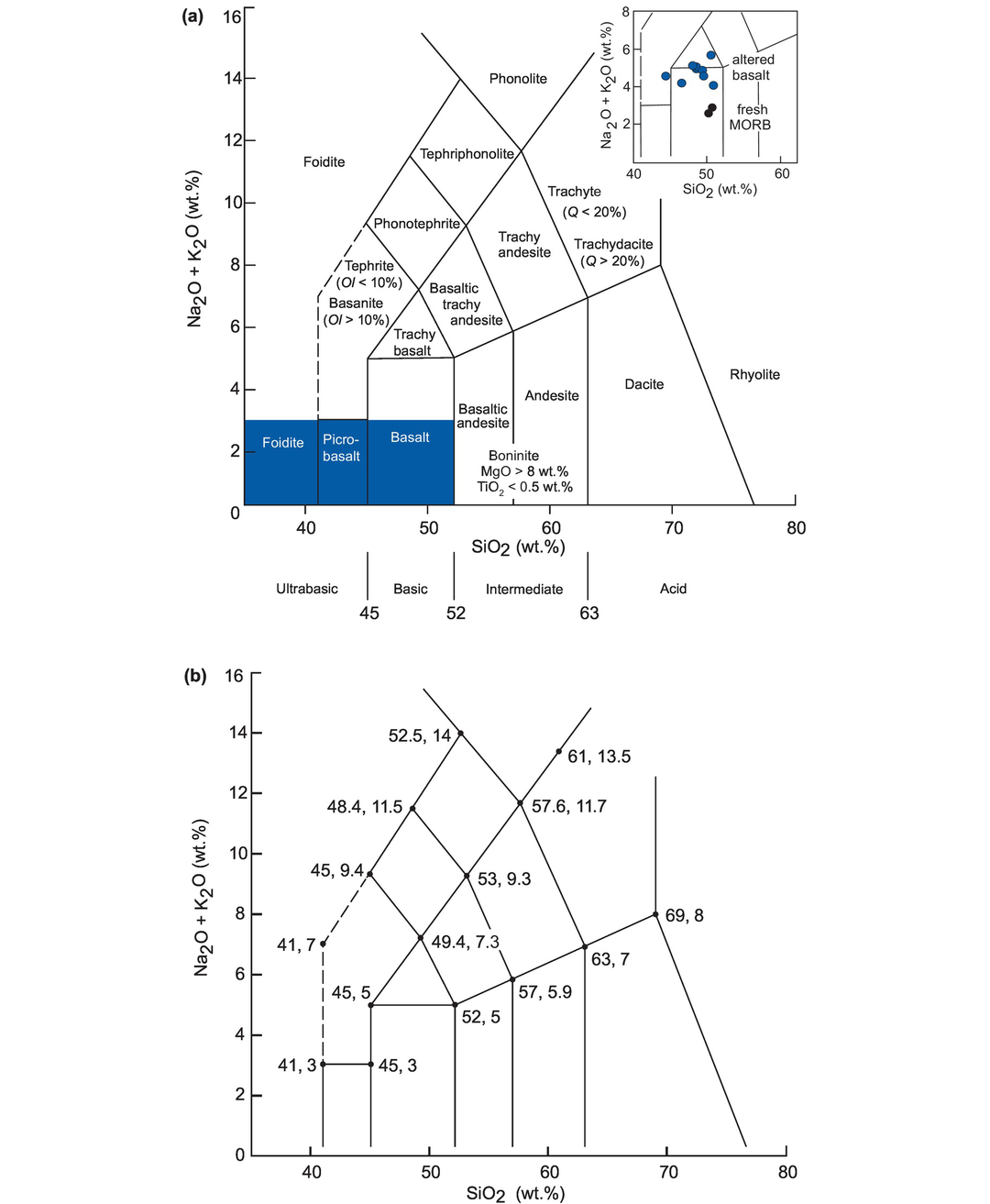
The total alkalis versus silica (TAS) diagram for volcanic rocks. (a) The chemical classification and nomenclature of Le Maitre et al. (2002) after Le Bas et al. (1986). Q = normative quartz, Ol = normative olivine. Ol- and Px-rich rocks occur in the shaded region, which is expanded in Figure 3.8. The inset shows the possible Na-enrichment of Permian basalts from Sumatra relative to fresh MORB. (b) Plotting coordinates for the field boundaries expressed as ‘SiO2 and (Na2O + K2O)’ after Le Bas et al. (1986).
| 1 | 2 | 3 | 4 | 5 | 6 | 7 | 8 | 9 | |
|---|---|---|---|---|---|---|---|---|---|
| Measured compositions | |||||||||
| MR136 | MR137 | MR139 | IG5 | IG4 | MR150 | MR152 | MR153 | 95SM11 | |
| SiO2 | 45.13 | 44.82 | 46.31 | 37.60 | 46.01 | 42.70 | 43.64 | 40.76 | 48.03 |
| Al2O3 | 14.11 | 13.79 | 14.25 | 14.21 | 12.91 | 13.42 | 14.87 | 13.28 | 14.46 |
| Fe2O3T | 8.93 | 9.16 | 9.05 | 10.54 | 11.58 | 9.30 | 8.74 | 9.06 | 12.78 |
| MnO | 0.11 | 0.12 | 0.10 | 0.15 | 0.11 | 0.11 | 0.11 | 0.12 | 0.19 |
| MgO | 7.34 | 8.75 | 7.34 | 6.54 | 7.08 | 6.32 | 6.34 | 8.37 | 7.74 |
| CaO | 10.88 | 8.95 | 7.36 | 9.89 | 6.16 | 10.04 | 8.32 | 10.90 | 7.92 |
| Na2O | 4.00 | 4.09 | 5.04 | 3.83 | 3.70 | 4.54 | 4.24 | 3.58 | 3.46 |
| K2O | 0.72 | 0.67 | 0.28 | 0.15 | 0.10 | 0.10 | 0.19 | 0.18 | 1.10 |
| TiO2 | 1.29 | 1.42 | 1.32 | 1.31 | 1.70 | 1.57 | 1.33 | 1.19 | 1.35 |
| P2O5 | 0.68 | 0.87 | 0.81 | 0.75 | 1.29 | 1.22 | 0.85 | 0.61 | 0.23 |
| LOI | 6.77 | 7.07 | 7.39 | 12.02 | 7.83 | 9.88 | 10.41 | 10.60 | 2.65 |
| Recalculated dry to 100% | |||||||||
| SiO2 | 48.43 | 48.38 | 50.41 | 44.25 | 50.76 | 47.81 | 49.24 | 46.29 | 49.38 |
| Al2O3 | 15.14 | 14.89 | 15.51 | 16.72 | 14.24 | 15.02 | 16.78 | 15.08 | 14.87 |
| Fe2O3T | 9.58 | 9.89 | 9.85 | 12.40 | 12.78 | 10.41 | 9.86 | 10.29 | 13.14 |
| MnO | 0.12 | 0.13 | 0.11 | 0.18 | 0.12 | 0.13 | 0.13 | 0.14 | 0.20 |
| MgO | 7.88 | 9.45 | 7.99 | 7.70 | 7.81 | 7.08 | 7.15 | 9.51 | 7.96 |
| CaO | 11.67 | 9.66 | 8.01 | 11.64 | 6.80 | 11.24 | 9.39 | 12.38 | 8.14 |
| Na2O | 4.29 | 4.42 | 5.49 | 4.51 | 4.08 | 5.08 | 4.78 | 4.07 | 3.56 |
| K2O | 0.77 | 0.72 | 0.30 | 0.18 | 0.11 | 0.11 | 0.21 | 0.20 | 1.13 |
| TiO2 | 1.38 | 1.53 | 1.44 | 1.55 | 1.88 | 1.75 | 1.50 | 1.35 | 1.39 |
| P2O5 | 0.73 | 0.94 | 0.88 | 0.88 | 1.42 | 1.37 | 0.96 | 0.69 | 0.24 |
| 100.00 | 100.00 | 100.00 | 100.00 | 100.00 | 100.00 | 100.00 | 100.00 | 100.00 | |
3.1.3 The Compositions of Some Major Earth Reservoirs
It is sometimes useful for comparison or normalisation to have representative values of some of the major Earth reservoirs. These are summarised in Table 3.2 for the major elements and in Table 4.9 for trace elements. Table 3.2a shows major element compositional data for the whole Earth (or the bulk Earth), the silicate Earth (or the bulk silicate Earth, or BSE, a term interchangeable with primitive upper mantle, or PM) and the Earth’s core. The data are expressed in wt.% elemental concentrations and oxygen is shown separately. This is because the core contains no oxygen and so expressing the data as elemental concentrations allows comparisons to be made between the silicate Earth and the core. In addition to the 10 major elements present in most silicate rocks, the metals Ni and Cr and the light elements H, C and S are also included as they constitute a measurable fraction of the composition of the whole Earth. These data are from McDonough (2014a) and assume that the original undifferentiated Earth was similar in composition to carbonaceous chondritic meteorites. It is known that the Earth’s core contains a few wt.% of a light element in addition to Fe and Ni, and the McDonough (2014a) model presented here argues that the principal light element is Si, but that there is also some S present.
| Bulk Earth | BSE/ primitive mantle | Earth's core | |
|---|---|---|---|
| Ref | 1 | 1 | 1 |
| Si | 16.100 | 21.000 | 6.000 |
| Ti | 0.081 | 0.120 | 0.000 |
| Al | 1.590 | 2.350 | 0.000 |
| Fe | 32.000 | 6.260 | 85.500 |
| Mn | 0.080 | 0.105 | 0.030 |
| Mg | 15.400 | 22.800 | 0.000 |
| Ca | 1.710 | 2.530 | 0.000 |
| Na | 0.180 | 0.270 | 0.000 |
| K | 0.016 | 0.024 | 0.000 |
| P | 0.072 | 0.009 | 0.200 |
| Ni | 1.820 | 0.196 | 5.200 |
| Cr | 0.470 | 0.263 | 0.900 |
| O | 29.700 | 44.000 | 0.000 |
| H | 0.026 | 0.010 | 0.060 |
| C | 0.073 | 0.012 | 0.200 |
| S | 0.635 | 0.025 | 1.900 |
| Total | 99.953 | 99.973 | 99.990 |
Reference: 1, McDonough (2014a).
| BSE/ primitive mantle | BSE/ primitive mantle | Depleted mantle | Mean MORB (whole rock) | Mean MORB (glass) | Mean continental crust | Mean upper continental crust | Mean middle continental crust | Mean lower continental crust | |
|---|---|---|---|---|---|---|---|---|---|
| Ref | 1 | 2 | 3 | 4 | 4 | 5 | 5 | 5 | 5 |
| SiO2 | 44.91 | 45.40 | 44.71 | 50.06 | 50.60 | 60.60 | 66.60 | 63.50 | 53.40 |
| TiO2 | 0.16 | 0.21 | 0.13 | 1.52 | 1.67 | 0.72 | 0.64 | 0.69 | 0.82 |
| Al2O3 | 4.44 | 4.49 | 3.98 | 15.00 | 14.79 | 15.90 | 15.40 | 15.00 | 16.90 |
| FeOT | 8.05 | 8.10 | 8.18 | 10.36 | 10.46 | 6.71 | 5.04 | 6.02 | 8.57 |
| MnO | 0.13 | 0.14 | 0.13 | 0.19 | 0.19 | 0.10 | 0.10 | 0.10 | 0.10 |
| MgO | 37.81 | 36.77 | 38.73 | 7.71 | 7.42 | 4.66 | 2.48 | 3.59 | 7.24 |
| CaO | 3.54 | 3.65 | 3.17 | 11.46 | 11.38 | 6.41 | 3.59 | 5.25 | 9.59 |
| Na2O | 0.36 | 0.35 | 0.13 | 2.52 | 2.77 | 3.07 | 3.27 | 3.39 | 2.65 |
| K2O | 0.03 | 0.031 | 0.006 | 0.190 | 0.190 | 1.810 | 2.800 | 2.300 | 0.610 |
| P2O5 | 0.02 | 0.020 | 0.019 | 0.160 | 0.180 | 0.130 | 0.150 | 0.150 | 0.100 |
| Total | 99.46 | 99.16 | 99.19 | 99.17 | 99.65 | 100.11 | 100.07 | 99.99 | 99.98 |
| Mg# | 89.3 | 89.0 | 89.4 | 59.0 | 58.0 | 55.3 | 46.7 | 51.5 | 60.1 |
| Xenolith Average | PUM | PUM | PUM | PUM | |
|---|---|---|---|---|---|
| Ref | 1 | 2 | 3 | 4 | 5 |
| SiO2 | 44 | 45.96 | 45.14 | 46.2 | 44.92 |
| Al2O3 | 2.27 | 4.06 | 3.97 | 4.75 | 4.44 |
| FeO | 8.43 | 7.54 | 7.82 | 7.7 | 8.05 |
| MgO | 41.4 | 37.78 | 38.3 | 35.5 | 37.8 |
| CaO | 2.15 | 3.21 | 3.5 | 4.36 | 3.54 |
| Na2O | 0.24 | 0.33 | 0.33 | 0.4 | 0.36 |
| K2O | 0.05 | 0.03 | 0.03 | nd | 0.29 |
| Cr2O3 | 0.39 | 0.47 | 0.46 | 0.43 | 0.38 |
| MnO | 0.14 | 0.13 | 0.14 | 0.13 | 0.14 |
| TiO2 | 0.09 | 0.181 | 0.217 | 0.23 | 0.201 |
| NiO | 0.012 | 0.28 | 0.27 | 0.23 | 0.25 |
| CoO | 0.014 | 0.013 | 0.013 | 0.012 | nd |
| P2O5 | 0.06 | 0.02 | nd | nd | 0.02 |
Table 3.2b provides the major element compositions of the major silicate reservoirs. The magnesium number (Mg#), its meaning and calculation are discussed in Section 3.3.2.1. As shown above, the primitive mantle is the same as the bulk silicate Earth – the Earth after the separation of the core but before the development of continental crust. Using the Earth reservoir data from Table 3.2a converted to oxide wt.%, the models of McDonough (2014a) and Palme and O’Neill (2014) are provided. The composition of the depleted mantle (DM) calculated by Workman and Hart (2005) is given for comparison and represents mantle from which some basaltic melt has been extracted. The DM, relative to PM, is more magnesian and slightly depleted in elements such as Ca, Al and Si which are preferentially incorporated into basaltic melt. A mean composition of over 2000 mid-ocean ridge basalt (MORB) samples from the floor of the major oceans is given and is very slightly different from the mean value of over 3000 MORB glass samples (data from White and Klein, 2014). Note, however, that these compositions simply represent what is found on the floor of the oceans and does not necessarily represent a primitive or primary MORB composition. The mean composition of the continental crust calculated by Rudnick and Gao (2014) is a weighted composite of the compositions of the upper, middle and more mafic lower continental crust.
Another important major Earth reservoir is the continental lithospheric mantle (CLM), often referred to in the literature as the sub-continental lithospheric mantle (SCLM) (see Table 3.2c). Fragments of the mantle provide our only direct samples of the CLM and include orogenic peridotites, ophiolites, and xenoliths transported via volcanism. Mantle xenoliths broadly define two compositional types: spinel- and garnet-facies peridotites associated with kimberlites, and spinel-facies peridotites associated with predominantly alkalic rocks. The former are generally found in cratonic settings and the latter in non-cratonic (rift) settings. Table 3.2c shows a compilation of xenolith and primitive upper mantle (PUM) model compositions from Pearson et al. (2014).
3.2 Rock Classification
With the advent of automated XRF and rapid ICP analytical methods most geochemical investigations produce a large volume of elemental data that allows for the classification of rocks on the basis of their chemical composition. This section reviews the classification schemes in current use and outlines the rock types for which they may be specifically suited. A summary of the classification schemes discussed is given in Box 3.1. We adhere to the guidelines of the International Union of Geological Sciences Sub-commission on the Systematics of Igneous Rocks (Le Maitre et al., 2002) for the naming and classification of rocks. We concur that a classification scheme should be easy to use, widely applicable, have a readily understood logical basis and reflect as accurately as possible the existing nomenclature based upon mineralogical criteria.
Igneous rocks
3.2.1 Oxide-oxide plots
The total alkalis-silica diagram (TAS)
for volcanic rocks
for plutonic rocks
for discriminating between the alkaline and sub-alkaline rock series
Subdivision of sub-alkalic volcanic rocks using K2O versus SiO2
3.2.2 NORM-based classifications
Basalt classification using the Ne–Di–Ol–Hy–Q diagram
Granite classification using the Ab–An–Or diagram
3.2.3 Cation classifications
Komatiitic, tholeiitic and calc-alkaline volcanic rocks using the Jensen plot
High-Mg rocks using the Hanski plot
3.2.4 Combined major element oxide and cation classification for granitoids
The Frost diagrams
Sedimentary rocks
3.2.5 The chemical classification of sedimentary rocks
Sandstones
Mudrocks
Limestones
3.2.1 Classifying Igneous Rocks Using Oxide-Oxide Plots
Bivariate oxide-oxide major element plots are the most straightforward way in which to classify igneous rocks, especially volcanic rocks, and the principal diagrams are summarised below.
3.2.1.1 The Total Alkalis-Silica Diagram (TAS) for Volcanic Rocks
The total alkalis-silica diagram is one of the most useful classification schemes available for volcanic rocks. Using wt.% oxide chemical data from a rock analysis that has been recalculated to 100% on an anhydrous (volatile-free) basis, the sum of Na2O + K2O (total alkalis, TA) and SiO2 (S) are plotted onto the classification diagram. The original version of the diagram (Le Bas et al., 1986) was expanded by Le Maitre et al. (1989) using 24,000 analyses of fresh volcanic rocks (Figure 3.1a). Le Maitre et al. (2002) further expanded the classification to include olivine- and pyroxene-rich rocks (Section 3.2.3.3).
The field boundaries were defined by minimizing the overlap between adjoining fields, and the boundary coordinates are given in Figure 3.1b. The TAS diagram divides rocks into ultrabasic, basic, intermediate and acid on the basis of their silica content following the usage of Peccerillo and Taylor (1976). The nomenclature is based upon a system of root names with additional qualifiers to be used as necessary. For example, the root name ‘basalt’ may be qualified to ‘alkali basalt’ or ‘sub-alkali basalt’. Some rock names cannot be allocated until the normative mineralogy has been determined. For example, a tephrite contains less than 10% normative olivine, whereas a basanite contains more than 10% normative olivine (see Section 3.2.2 on the norm calculation).
The TAS classification scheme is intended for common volcanic rocks and should not be used with weathered, altered or metamorphosed volcanic rocks because the alkali elements can be mobilised. Potash-rich rocks (nephelinites, mela-nephelinites) should not be plotted on the TAS diagram, and ultramafic or high-Mg rocks (boninite, komatiite, meimechite, picrite) should be checked for their TiO2 contents before assigning a name from the TAS diagram (see Section 3.2.3.3). Rocks showing obvious signs of crystal accumulation should also be avoided.
3.2.1.2 A TAS Diagram for Plutonic Rocks
Of the various schemes for the naming of plutonic rocks, the two most popular ones based on major element chemistry are the TAS diagram for plutonic igneous rocks (after Wilson, 1989) and the normative Q–Or–Ab triangular plot for granitoids (Section 3.3.2). The TAS diagram for plutonic rocks (Figure 3.2) is useful inasmuch as it is simple and convenient to use. It is important to note, however, that its boundaries are not the same as the boundaries of the TAS diagram for volcanic rocks. There are other classification schemes for plutonic rocks which are based on modal mineralogy, but these are not discussed here.

3.2.1.3 Discrimination between the Alkalic and Sub-alkalic Rock Series Using TAS
Igneous rocks can be subdivided into an alkalic or sub-alkalic magma series on the TAS diagram. Using data from Hawaiian basalts, MacDonald and Katsura (1964) were the first to define a boundary separating the alkalic and sub-alkalic (tholeiitic) magma series on a TAS diagram. A later study by MacDonald (1968) expanded the boundary to cover a wider range of SiO2. Similar diagrams by Kuno (1966) and Irvine and Baragar (1971) place the boundary in slightly different positions on the TAS plot (Figure 3.3). Currently, the boundary curve of Irvine and Baragar (1971) is the most widely used, although the recent reassessment by El-Hinnawi (2016a) indicates that the coordinates of MacDonald and Katsura (1964) provide the best distinction between the alkalic and sub-alkalic series for basaltic compositions (SiO2 < 52 wt.%). There is less clarity for compositions with a higher SiO2 content. The boundary coordinates are given in the caption to Figure 3.3.
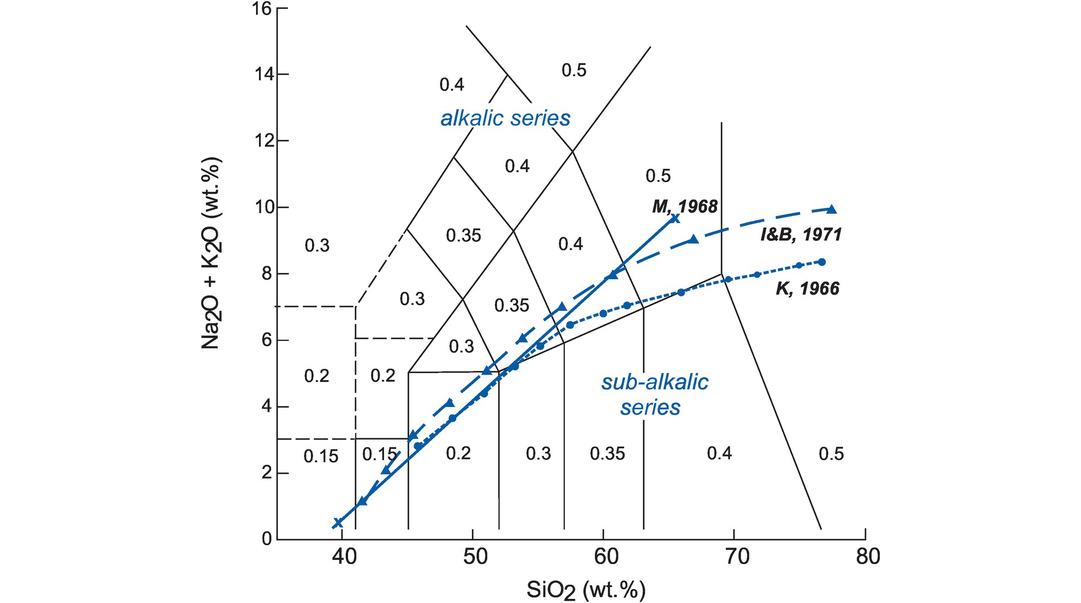
The TAS diagram for volcanic rocks showing (i) subdivisions between the alkalic and sub-alkalic magma series and (ii) the Fe2O3/FeO ratios for volcanic rock compositions recommended by Middlemost (1989). Note: Boundaries and plotting coordinates (SiO2, total alkalis) are, respectively, from Kuno (1966 – K, 1966 – filled circles [dotted line 45.85, 2.75; 46.85, 3.0; 50.0, 3.9; 50.3, 4.0; 53.1, 5.0; 55.0, 5.8; 55.6, 6.0; 60.0, 6.8; 61.5, 7.0; 65.0, 7.35; 70.0, 7,85; 71.6, 8.0; 75.0, 8.3; 76.4, 8.4]); MacDonald (1968 – M, 1968 – crosses [solid line 39.8, 0.35 to 65.5, 9.7]) and Irvine and Baragar (1971 – I&B, 1971 – filled triangles [dashed line 39.2, 0.0; 40.0, 0.4; 43.2, 2.0; 45.0, 2.8; 48.0, 4.0; 50.0, 4.75; 53.7, 6.0; 55.0, 6.4; 60.0, 8.0; 65.0, 9.6; 66.4, 10.0]). The data are from the compilation of Rickwood (1989). Note the greater divergence between the boundaries at higher SiO2.
Alkaline plutonic rocks enriched in magnesium are known as sanukitoids. They were originally defined by Stern et al. (1989) as plutonic rocks containing 55–60 wt.% SiO2 and with Mg# > 0.6 (see Section 3.3.2). However, it is now known that there are sanukitoid suites which range in composition from pyroxenite to quartz monzonite with SiO2 between 38 wt.% and 68 wt.% and Mg# = 0.49–0.89. This is illustrated in the study by Lobach-Zhuchenko et al. (2008, figure 4).
3.2.1.4 The K2O versus SiO2 Diagram for the Sub-division of the Sub-alkalic Series
Volcanic rocks of the sub-alkalic series may be further subdivided into the calc-alkalic or tholeiitic series on the basis of their K2O and SiO2 concentrations (Peccerillo and Taylor, 1976). Le Maitre et al. (1989) proposed a subdivision of sub-alkalic rocks into low-, medium- and high-K types and suggested that these terms be used to qualify the names ‘basalt’, ‘basaltic andesite’, ‘andesite’, ‘dacite’ and ‘rhyolite’. This nomenclature broadly coincides with the low-K (tholeiitic) series, medium-K (calc-alkalic) series and high-K (calc-alkaline) series of Rickwood (1989). A compilation of curves from Rickwood (1989) and Le Maitre et al. (1989) is given in Figure 3.4.
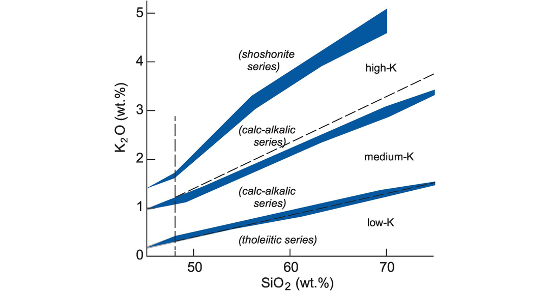
The subdivision of alkalic and sub-alkalic rocks using the K2O versus silica diagram. The diagram shows the subdivisions of Le Maitre et al. (1989) (dashed lines and upper case text) and of Rickwood (1989) (text in parentheses). The shaded regions include the boundaries of Peccerillo and Taylor (1976), Ewart (1982), Innocenti et al. (1982), Carr (1985) and Middlemost (1985) as summarised by Rickwood (1989). The plotting parameters are as follows (SiO2, K2O): Le Maitre et al. (1989): (dashed lines) high-K/medium-K boundary 48.0, 1.2; 68.0, 3.1; medium-K/low-K boundary 48.0, 0.3; 68.0, 1.2; vertical boundary at 48 wt.% SiO2. Rickwood (1989): the band between the shoshonitic series and the high-K series 45.0, 1.38; 48.0, 1.7; 56.0, 3.3; 63.0, 4.2; 70.0, 5.1; and 45.0, 1.37; 48.0, 1.6; 56.0, 2.98; 63.0, 3.87; 70.0, 4.61; the band between the high-K and the calc-alkalic series 45.0, 0.98; 49.0, 1.28; 52.0, 1.5; 63.0, 2.48; 70.0, 3.1; 75.0, 3.43; and 45.0, 0.92; 49.0, 1.1; 52.0, 1.35; 63.0, 2.32; 70.0, 2.86; 75.0, 3.25; the band between the calc-alkalic and the low-K series 45.0, 0.2; 48.0, 0.41; 61.0, 0.97; 70.0, 1.38; 75.0, 1.51; and 45.0, 0.15; 48.0, 0.3; 61.0, 0.8; 70.0, 1.23; 75.0, 1.44.
3.2.2 Classifying Igneous Rocks Using Normative Mineralogy
The norm represents a theoretical mineral assemblage which is calculated from a whole rock chemical analysis. In the context of rock classification it provides the basis for a number of mineralogical classification schemes. The calculated normative mineralogy is based entirely upon the chemistry of the rock and its strength lies in the fact that it permits the classification of rocks, such as glassy rocks, for which the determination of the mode is not possible, and allows a direct comparison to be made between such rocks and their crystalline or metamorphosed counterparts. Hence rocks with the same chemical composition should result in the same normative mineral assemblage, although it is important to note that the norm calculation is sensitive to the oxidation state of iron (see Section 3.2.2.3).
3.2.2.1 CIPW Norm
There are a number of different approaches to calculating the norm but the CIPW norm, named after its originators – Cross, Iddings, Pirrson and Washington (Cross et al., 1902) – is the most commonly used. The CIPW norm calculation makes a number of simplifying assumptions and follows a prescribed set of rules. A simplified version of the calculation scheme is given in Appendix 3.1. An example of the conversion steps needed to calculate molar proportions necessary to determine the norm is given in Table 3.3. Weight percent oxide values (column 1) are divided by their molecular weights (column 2) to calculate molecular proportions (column 3). The molecular proportions are the basis of the norm calculation given in Appendix 3.1. At the end of the calculation the resulting normative minerals are multiplied by their molecular weight to recast them into wt.% (column 9). The CIPW norm calculation can be carried out in Excel using the programme norm 4 (https://minerva.union.edu/hollochk/c_petrology/other_files/norm_calculation.pdf) or in a variety of open-source computer programs such as NORRRAM (González-Guzmán, 2016, in R) or CIPWFULL (Al-Mishwat, 2015, in FORTRAN). However, it is important to understand the principles which lie behind the norm calculation, and so before using these programs we recommend the manual calculation of a simple CIPW norm.
| 1 | 2 | 3 | 4 | 5 | 6 | 7 | 8 | 9 | 10 | ||
|---|---|---|---|---|---|---|---|---|---|---|---|
| Wt.% oxide of rock | Mol. wt. | Mol. proportions | Number of cations | Cation proportions | Millications | Cation % | Mole % | Normative minerals | CIPW norm | Cation norm | |
| SiO2 | 61.52 | 60.09 | 1.0238 | 1 | 1.0238 | 1023.80 | 58.03 | 67.86 | Q | 15.94 | 15.12 |
| TiO2 | 0.73 | 79.9 | 0.0091 | 1 | 0.0091 | 9.14 | 0.52 | 0.61 | Or | 12.23 | 12.45 |
| Al2O3 | 16.48 | 101.96 | 0.1616 | 2 | 0.3233 | 323.26 | 18.32 | 10.71 | Ab | 30.71 | 33.2 |
| Fe2O3 | 1.83 | 159.69 | 0.0115 | 2 | 0.0229 | 22.92 | 1.30 | 0.76 | An | 22.52 | 22.98 |
| FeO | 3.82 | 71.85 | 0.0532 | 1 | 0.0532 | 53.17 | 3.01 | 3.52 | Di | 2.17 | 2.18 |
| MnO | 0.08 | 70.94 | 0.0011 | 1 | 0.0011 | 1.13 | 0.06 | 0.07 | Hy | 10.32 | 10.47 |
| MgO | 2.8 | 40.3 | 0.0695 | 1 | 0.0695 | 69.48 | 3.94 | 4.61 | Mt | 2.64 | 1.95 |
| CaO | 5.42 | 56.08 | 0.0966 | 1 | 0.0966 | 96.65 | 5.48 | 6.41 | Il | 1.38 | 1.04 |
| Na2O | 3.63 | 61.98 | 0.0586 | 2 | 0.1171 | 117.13 | 6.64 | 3.88 | Ap | 0.56 | 0.53 |
| K2O | 2.07 | 94.2 | 0.0220 | 2 | 0.0439 | 43.95 | 2.49 | 1.46 | |||
| P2O5 | 0.25 | 141.95 | 0.0018 | 2 | 0.0035 | 3.52 | 0.20 | 0.12 | TOTAL | 98.47 | 99.92 |
| TOTAL | 98.63 | 1.7641 | 100.00 | 100 | An | 34% | 33% | ||||
| Ab | 47% | 48% | |||||||||
| Or | 19% | 18% |
The CIPW norm is widely used in the classification of basalts (Section 3.2.2.4) and in the classification of granitoids (Section 3.2.2.5). Errors can arise in CIPW norm calculations if volatiles in the rock composition are not correctly allocated and if the oxidation state of the iron is incorrectly stated. In addition, some rock types, in particular, cumulate rocks and alkaline rocks with a high CO2 content, may result in the calculation of an improbable range of accessory mineral phases.
3.2.2.2 The Cation Norm
The Barth-Niggli norm, also known as the cation norm or the molecular norm, is an older norm calculation that is no longer widely used. The norm is calculated using the equivalent weights of the oxides, that is, the molecular weight when one cation is present (Barth, 1952). In the case of oxides such as CaO or TiO2 the equivalent weight is the same as the molecular weight, but for Al2O3 or Na2O the equivalent weight is half the molecular weight. The calculation of a cation norm is illustrated in Table 3.3. In this case the wt.% oxide values (column 1) are divided by their equivalent weights (divide by column 2 and multiply by column 4), converted into cation proportions (column 5) and then converted into cation percent (column 7). Molecules are then constructed according to the standard CIPW rules (Appendix 3.1), although the proportions of the components in which cations are allocated are different from the CIPW norm. The cation norm is not recalculated on a wt.% basis, but is expressed in molecular % (column 10). One advantage of the cation norm is that the proportions of opaque minerals are closer to their volume percentages as seen in thin section.
3.2.2.3 Normative Mineralogy and the Oxidation State of Iron
The norm calculation is particularly sensitive to the oxidation state of iron. This is problematic for mafic rocks where the Fe content is typically much higher than in felsic rocks, and can be an issue for felsic rocks since magmatic systems generally become more oxidising as they evolve. Given that Fe is usually reported as either FeO or as Fe2O3 it is necessary to estimate the Fe2O3/FeO ratio in a given rock. Two approaches have been taken. In volcanic rocks, Middlemost (1989) assigned specific values of Fe2O3/FeO to particular rock types in TA-S space (Figure 3.3). El-Hinnawi (2016b), on the other hand, used a database of >12,000 analyses for which Fe was measured as Fe2+ and Fe3+ to directly calculate the Fe2O3/FeO ratio. This study showed that there is a linear relationship between total alkalis (Na2O + K2O) and the degree of iron oxidation (OxFe = Fe2O3/(Fe2O3 + FeO) in wt.%) in the alkalic and sub-alkalic volcanic rock series (Figure 3.5). The equations are:
These results are applicable to the majority of volcanic rock types, although ‘transitional’ basalts with compositions between the two fields are more difficult to constrain.
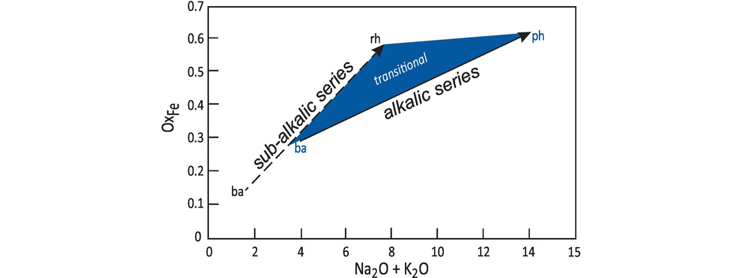
Average degree of iron oxidation (OxFe = Fe2O3/(Fe2O3 + FeO)) associated with total alkalis of the alkalic and sub-alkalic volcanic rock series (after El-Hinnawi, 2016b). As a magma evolves towards more sialic differentiates, the increase in oxygen fugacity leads to an increase in iron oxidation, resulting in the strong positive correlation for both the alkalic (solid arrow) and sub-alkalic (dashed arrow) series. The arrows indicate direction of evolution from basaltic (ba) to rhyolitic (rh)/phonolitic (ph) compositions. The shaded area indicates region of ‘transitional’ basalts, which will have intermediate OxFe.
Given the widespread use of normative mineralogy in classifying basaltic and granitic rocks and the impact the oxidation state of Fe can have on the normative mineralogy, it is necessary to specify how Fe has been allocated between its two oxidation states when reporting the results of norm calculations.
3.2.2.4 Normative Mineralogy and Basalt Classification
Thompson (1984) proposed a classification scheme for basaltic rocks based upon the CIPW normative proportions of Ne (and other feldspathoids), Ol, Di, Hy and Q (see Appendix 3.1 for abbreviations). This classification diagram (Figure 3.6) is an expanded version of the Yoder-Tilley (1962) low-pressure basalt tetrahedron (Figure 3.22a). The three equilateral triangles of the diagram Ne–Ol–Di, Ol–Di–Hy and Di–Hy–Q represent basaltic and related rocks which are, respectively, undersaturated, saturated and oversaturated with silica (Figure 3.6). Thus silica undersaturated basalts (alkali basalts) are characterised by normative Ol and Ne, silica saturated basalts (olivine tholeiites) are characterised by normative Hy and Ol, and silica oversaturated basalts (quartz tholeiites) are characterised by normative Q and Hy.
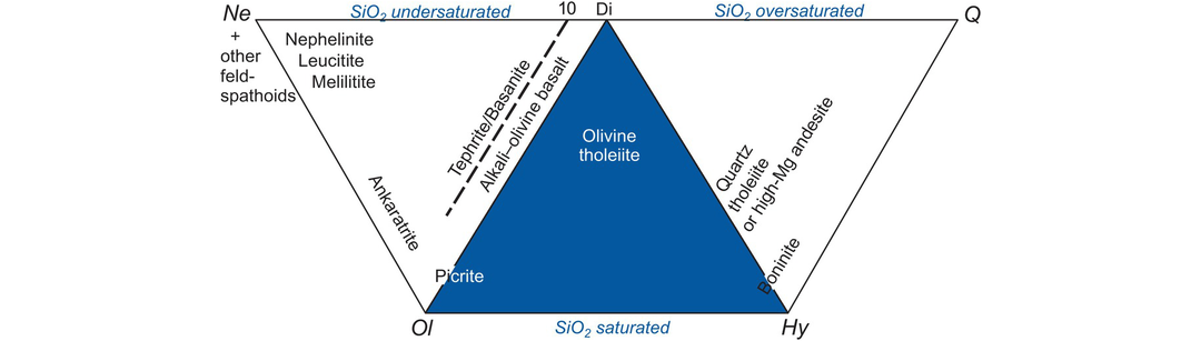
The classification of basalts and related rocks based upon their CIPW normative compositions expressed as Ne–Ol–Di, Ol–Di–Hy or Di–Hy–Q.
Silica saturation is particularly important in basaltic magmas, because in dry magmas this single parameter determines the crystallisation sequence of minerals and evolution of the melt during fractional crystallisation. Weight % normative compositions (calculated assuming FeO/(FeO + Fe2O3) = 0.85, or Fe2O3/FeO = 0.18) are projected onto one of the three triangles by summing the three relevant normative parameters and calculating the value of each as a percentage of their sum. The calculation and plotting procedure for triangular diagrams is given in Section 3.3.3. This diagram is intended to be used with basalts which have MgO > 6 wt.% and should not be used for highly evolved magmas. Disadvantages of this classification are that it uses only about half of the calculated norm and so is not fully representative of the rock chemistry. It is also sensitive to small errors in Na2O and so is inappropriate for altered rocks.
3.2.2.5 Normative Mineralogy and Granite Classification
The Ab–An–Or normative classification diagram of Barker (1979) modified from O’Connor (1965) provides a convenient way of classifying felsic plutonic rocks on the basis of their major element chemistry (Figure 3.7). The normative calculation provides a more accurate estimate of feldspar compositions than a modal classification, for it reflects solid solution in the feldspars. The An–Ab–Or diagram represents a projection from quartz onto the feldspar face of the normative ‘granite’ tetrahedron Q–Ab–An–Or. The diagram can be applied to felsic rocks with more than 10% normative quartz and is based entirely upon the normative feldspar composition recast to 100%. The feldspar compositions in this classification were originally calculated using the Barth-Niggli molecular norm, although it is not clear whether this procedure has been followed by all users. That said, the plotting parameters in the Ab–An–Or projection are within 2% of each other from either norm calculation scheme; this is illustrated in Table 3.3 where the Ab–An–Or plotting parameters for a tonalite are calculated using both the CIPW and the molecular norm. Field boundaries of the original O’Connor (1965) diagram were empirically defined from a dataset of 125 plutonic rocks for which there was both normative and modal data. Barker’s (1979) revised classification has the advantage of field boundaries which are clear and easy to reproduce, and which effectively separate tonalites, trondhjemites, granites and granodiorites from each other. The diagram can also be used (with caution) for deformed and metamorphosed granitic rocks, permitting an estimate of their original magma type.
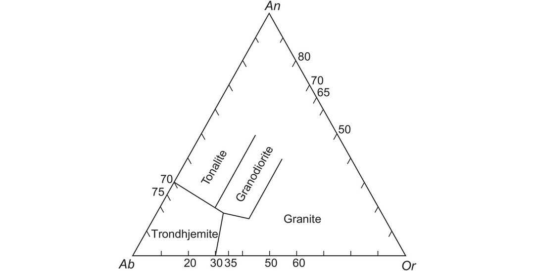
The classification of ‘granitic’ rocks according to their molecular normative An–Ab–Or composition after Barker (1979).
3.2.3 Classifying Igneous Rocks Using Cations
The conversion of wt.% oxides to cations is calculated in the same way as in the initial stages of the cation norm calculation. The wt.% of the oxide is divided by the equivalent weight of the oxide set to one cation. It is sometimes alternatively expressed as the wt.% oxide divided by the molecular weight of the oxide and multiplied by the number of cations in the formula unit. Thus the wt.% SiO2 is divided by 60.09. However, the wt.% Al2O3 is divided by 101.96 and then multiplied by 2. If millications are needed, then multiply the cationic proportions by 1000. Worked examples are given in columns 5 and 6 of Table 3.3.
3.2.3.1 The Jensen Plot
Jensen (1976) proposed a cation-based classification scheme for sub-alkalic volcanic rocks. It is based upon the cation proportions of Σ(Fe2+ + Fe3+ + Ti), Al and Mg recalculated to 100% and plotted on a triangular diagram (Figure 3.8b). The elements were selected on the basis of their variability in sub-alkalic rocks, for the way in which they vary in inverse proportion to each other and for their stability under low grades of metamorphism. Thus, this classification scheme can be used successfully with metamorphosed volcanic rocks that have experienced mild metasomatic loss of alkalis – an advantage over other classification schemes for volcanic rocks. However, this diagram is important because it shows komatiites and komatiitic basalts as separate fields from those of basalts and calc-alkaline rocks and so is useful for Archean metavolcanic rocks. The original diagram of Jensen (1976) was slightly modified by Jensen and Pyke (1982), who moved the komatiitic basalt/komatiite field boundary to a lower value of Mg, and this is the version presented in Figure 3.8b. The plotting parameters of the field boundaries are taken from Rickwood (1989).
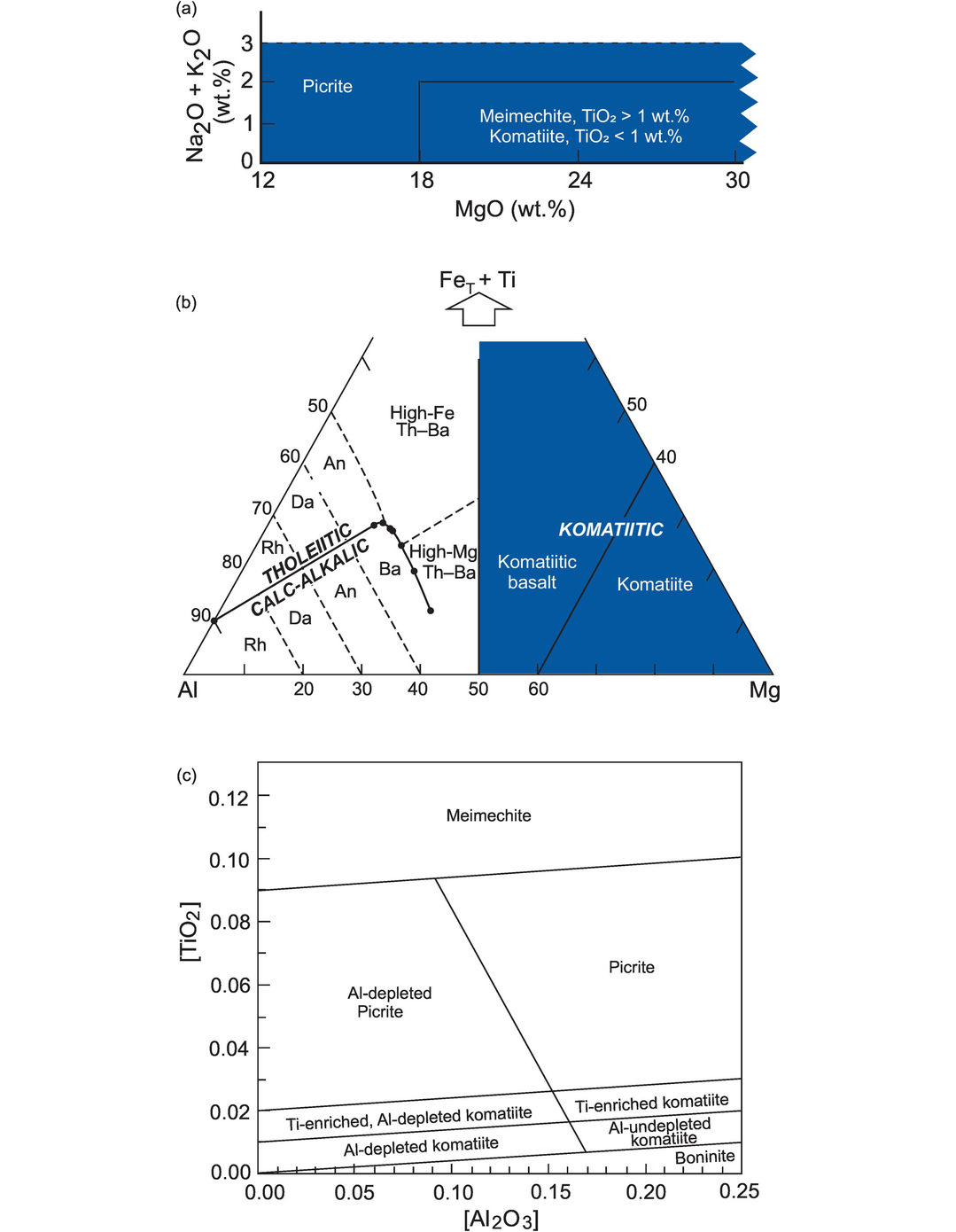
The classification of high-Mg volcanic rocks. (a) High-Mg rocks (shaded region in lower left of the TAS diagram in Figure 3.1) are further divided on the basis of their wt.% MgO and TiO2 (Le Maitre et al., 2002). (b) High-Mg basalts and komatiitic rocks are classified using cation percentages of Al, (Fe[total] + Ti) and Mg. The field boundaries are after Jensen (1976) and Jensen and Pyke (1982) (heavy lines). An, andesite; Ba, basalt; Da, dacite, Rh, rhyolite; Th, tholeiite. The boundary between the tholeiitic and calc-alkalic fields is defined by the coordinates (Al, Fe + Ti, Mg) 90, 10, 0; 53.5, 28.5, 18; 52.5, 29, 18.5; 51.5, 29, 19.5; 50.5, 27.5, 22; 50.3, 25, 24.7; 50.8, 20, 29.2; 51.5, 12.5, 36 (Rickwood, 1989; corrected). (c) High-Mg rocks classified using molecular proportions of Al2O3 and TiO2 normalised to unity using the equation [Al2O3] = Al2O3/(2/3 – MgO – FeO) and [TiO2] = (TiO2/(2/3 – MgO – FeO). (Hanski et al., 2001)
3.2.3.2 The Hanski Plot
The Hanski plot is also useful for distinguishing between high-Mg rocks (Figure 3.8c). The diagram is based upon the molecular proportions of Al2O3 and TiO2 (normalised to unity) and projected from olivine. All the iron is assumed to be ferrous (Hanski et al., 2001). The plotting parameters are as follows:
Figure 3.8c distinguishes between komatiites and picrites and between Al- and Ti-enriched/depleted komatiites. It has the advantage that rock or liquid compositions with an olivine-controlled liquid-line-of-descent will have constant [Al2O3] and [TiO2] values, thus a fixed position on the plot. However, the diagram does not distinguish between komatiites and komatiitic basalts.
3.2.3.3 Classification of High-Mg Rocks on the TAS Diagram
Although not a cation plot, it is relevant here to consider the classification of high-Mg rocks within the framework of the TAS diagram. Le Maitre et al. (2002) sought to differentiate between picrites and komatiites and other highly magnesian rocks on the basis of their MgO and TiO2 content (see the shaded region in Figures 3.1 and 3.8a).
3.2.4 A Combined Major Element Oxide and Cation Classification for Granitoids
We recommend a major element scheme for distinguishing between groups of granitoids. We suggest that this is superior to trace element classifications since these can be distorted by the accumulation of accessory mineral phases (Bea, 1996). The scheme proposed here is non-genetic and so lacks any assumption about the origin of the granitoid, thereby avoiding some of the pitfalls of the SIAM-type granite classification of Chappell and White (1974). Further it avoids the less-intuitive approach of the R1-R2 classification proposed by de la Roche et al. (1980).
Instead, we follow the classification scheme of Frost et al. (2001), modified by Frost and Frost (2008). The ‘Frost’ classification subdivides granitoids on the basis of five indices:
1. an iron index
2. a modified alkali-lime index (after Peacock, 1934)
5. a feldspathoid saturation index.
These parameters are summarised in Table 3.4, plotted in Figure 3.9 and discussed in more detail below.
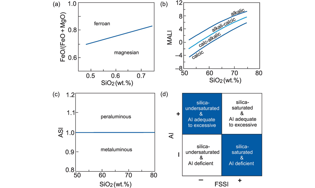
Granite classification using major elements (after Frost et al., 2001 and Frost and Frost, 2008). (a) The Fe-index distinguishes magnesian versus ferroan rocks on the basis of total iron in the rock calculated as wt.% Fe-index = FeO + 0.9Fe2O3/(FeO + 0.9Fe2O3 + MgO). This is similar to the ‘calc-alkalic’ and ‘tholeiitic’ trends of Miyashiro (1974). The boundary fits the equation FeO* = 0.46 + 0.005SiO2. (b) The modified alkali-lime index (MALI) reflects the wt.% relationship of Na2O + K2O – CaO relative to SiO2 and is a function of the crystallising assemblage. This index separates the alkalic, alkali-calcic, calc-alkalic and calcic rocks from one another. (c) The alumina saturation index (ASI) is based on molecular Al/(Ca – 1.67P + Na + K) and defines rocks as metaluminous (ASI < 1) or peraluminous (ASI > 1). (d) The combination of the molecular alkalinity index (AI) and the normative feldspathoid silica-saturation index (FSSI) identifies alkalic rocks, and SiO2-saturated or under-saturated rocks, respectively. AI = molecular Al/(Ca – 1.67P + Na + K) (after Shand, 1947); FSSI = normative Q − [Lc + 2(Ne + Kp)]/100.
| Index | Formula | Units | ||
|---|---|---|---|---|
| 1. Fe-index | FeO/(FeO+MgO) | Wt.% oxide | ||
| 2. Modified alkali-lime index (MALI) | Na2O + K2O – CaO | Wt.% oxide | ||
| 3. Aluminum-saturation Index (ASI) | Al/(Ca − 1.67P + Na + K) | Molecular | ||
| 4. Alkalinity index (AI) | Al − (K + Na) | Molecular | ||
| 5. Feldspathoid silica-saturation Index (FSSI) | Q − [Lc − 2(Ne + Kp)]/100 | Molecular norm | ||
The Fe-index separates those rocks enriched in Fe from those that are not and identifies them as ferroan or magnesian (Figure 3.9a). The index is calculated as FeO* = [FeO + 0.9 Fe2O3/(FeO + 0.9 Fe2O3 + MgO)] (wt.%) and the boundary between ferroan and magnesian rocks fits the equation [FeO* = 0.46 + 0.005 SiO2] (Frost and Frost, 2008).
The modified alkali-lime index (MALI) reflects the wt.% abundance of sodium and potassium relative to calcium using the equation Na2O + K2O - CaO. When the MALI index is plotted against SiO2 it distinguishes between alkalic, alkali-calcic, calc-alkalic and calcic compositions (Figure 3.9b). Rocks with more than ~ 60% SiO2 are controlled by the abundance and composition of feldspars and quartz; at lower SiO2, the removal of augite during fractionation exerts a dominant control on increasing MALI in the residual magma.
The aluminium saturation index (ASI) is based on molecular Al/(Ca - 1.67P + Na + K) and identifies rocks as metaluminous or peraluminous (after Shand, 1947; Zen, 1988) (Figure 3.9c). Peraluminous varieties (ASI > 1) have more Al than is needed to make feldspars (molecular Na + K < AI), whereas metaluminous varieties (ASI < 1) lack the necessary Al needed to make feldspars (molecular Na + K > AI). Alkaline rocks are deficient in either alumina or silica or both, and contain higher alkalis than can be accommodated in feldspar alone.
The alkalinity index (AI) and the feldspathoid silica-saturation index (FSSI) combine to discriminate between alkaline rocks on the basis of alumina relative to alkalis [AI = molecular Al - (K + Na)] as well as between silica-saturated and undersaturated compositions (Figure 3.9d). The FSSI is based on the molecular norm using the equation Q - [Lc + 2(Ne + Kp)]/100.
On the basis of these five indices, it is possible to classify the majority of granitoids.
3.2.5 The Chemical Classification of Sedimentary Rocks
Most sedimentary rock classification schemes use those features that can be observed in hand specimen or thin section. In clastic rocks these are grain size and the mineralogy of the grains and matrix (Milliken, 2014; Garzanti, 2019) and in limestones they are depositional textures (Dunham, 1962) or grain compositions (Folk, 1959).
The chemical composition of clastic rocks is a complex function of the composition of the protolith, mediated by the processes of weathering, transport, diagenesis and depositional environment. For this reason the bulk-rock chemistry of a clastic sediment is more useful in investigating processes such as hydraulic sorting, chemical weathering and the detrital mineralogy of the source than in rock classification (Johnsson, 1993; Mangold et al., 2011; Fedo et al., 2015). Nevertheless, there are now abundant, precise elemental data for both coarse- and fine-grained sedimentary rocks, and so, with the above caveats in mind, some applications associated with major element chemistry are presented below.
3.2.5.1 Sandstones
Sandstone geochemistry can be used to distinguish between mature and immature varieties using the relative abundances of quartz, feldspar + clay, and ferromagnesian minerals. Prolonged weathering breaks down ferromagnesian minerals and so depletes the sediment in Ti + Mg + Fe. In a similar way through the breakdown of feldspars and micas the sediment is depleted in K + Na. This gives rise to an increase in residual quartz (SiO2) and a high level of compositional maturity as illustrated in Figure 3.10a (Roser et al. 1996). Using these same principles for the classification of sandstones and shales, Herron (1988) plotted the parameters log (SiO2/Al2O3) against log(Fe2O3T/K2O) (Figure 3.10b). The ratio Fe2O3T/ K2O is a measure of the stability of ferromagnesian minerals and permits sandstones to be more successfully classified than simply using the K-Na scheme of Pettijohn et al. (1972). Shales are identified on the basis of their low SiO2/Al2O3. A further advantage of the Herron classification is that it can be used to identify shales, sandstones, arkoses and carbonate rocks in situ from geochemical well logs using neutron activation and gamma-ray tools (Herron and Herron, 1990). However, sediment classification diagrams based on major elements must be applied with caution as Na and K can be easily mobilised during diagenesis and metamorphism. The degree of chemical alteration can be evaluated using the alteration parameters listed in Table 3.5 and is discussed further in Section 3.3.
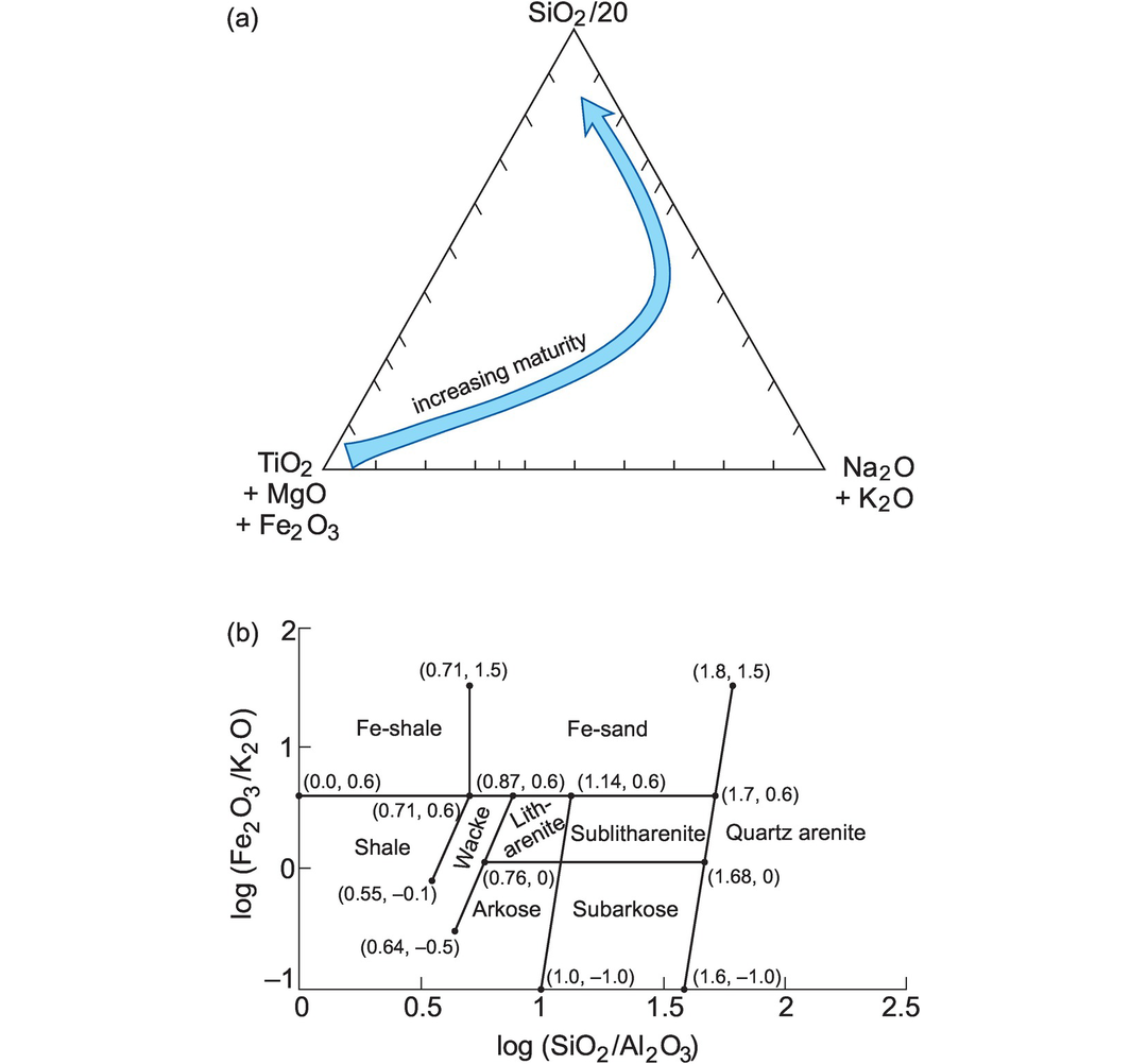
Major element classification of sediments. (a) Sandstone maturity as a function of wt.% SiO2/20, K2O + Na2O, and TiO2 + MgO + Fe2O3 (after Kroonenberg, 1990). The mature sandstones are nearest the SiO2 apex. (b) Terrigenous sandstones and shales in a log (Fe2O3/K2O) versus log (SiO2/Al2O3) plot (after Herron, 1988). The numbers shown in parentheses are the plotting coordinates for the field boundaries expressed as [log (SiO2/Al2O3), log (Fe2O3/K2O)].
| Index | Units | Reference |
|---|---|---|
| Index of compositional variability (ICV) | ||
| [Fe2O3 + K2O + Na2O + CaO + MgO + MnO + TiO2]/Al2O3 | Wt.% oxide | Cox et al. (1995) |
| Plagioclase index of alteration (PIA) | ||
| [(Al2O3 - K2O)/(Al2O3 + CaO + Na2O - K2O)] × 100 | Wt.% oxide | Fedo et al. (1995) |
| Chemical index of weathering (CIW) | ||
| [Al2O3/(Al2O3 + CaO + Na2O)] × 100 | Wt.% oxide | Harnois (1988) |
| Chemical index of weathering without CaO (CIW′) | ||
| Al2O3/(Al2O3 + Na2O) | Wt.% oxide | Cullers (2000) |
| Chemical index of alteration (CIA) | ||
| [Al2O3/(Al2O3 + CaO* + Na2O + K2O)] × 100 | Molar | Nesbitt and Young (1982) |
| Chemical proxy of alteration (CPA) | ||
| 100 × [Al2O3/(Al2O3 + Na2O)] | Molecular norm | Buggle et al. (2011) |
3.2.5.2 Mudrocks
There is no widely recognised major element chemical classification of mudrocks. This is surprising given that they have a more variable chemistry than sandstones. Whole-rock major element data are typically presented normalized to a reference composition such as the Post-Archean Australian Shale (PAAS) of Taylor and McLennan (1985). The index of compositional variability (ICV) ([Fe2O3 + K2O + Na2O + CaO + MgO + MnO + TiO2]/Al2O3) has also been used to indicate increasing or decreasing proportions of clay minerals on the basis that clay minerals have greater amounts of alumina (Cox et al., 1995). More recently Fazio et al. (2019) used Na2O versus SiO2 and Na2O versus Al2O3 (wt.%) to distinguish between varieties of mudrock.
3.2.5.3 Limestones
Most carbonate rocks are dominated by calcite, dolomite and their ferroan equivalents and contain only a limited amount of other constituents. Consequently, their major element chemistry is dominated by Ca, Mg and Fe (Figure 3.11). Limestones and marbles can be classified on the basis of their relative CaCO3 and MgCO3 content and divided into two main categories: magnesite (≥50% MgCO3) and calcite-dolomite [CaCO3–(Ca, Mg)CO3]. The calcite-dolomite group can be further subdivided into six categories on the basis of their purity (Carr and Rooney, 1983).
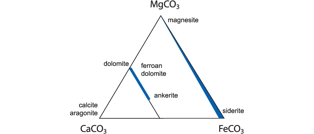
Carbonate rock classification. Carbonate minerals stable at sub-greenschist (<250°C ) conditions (data from Anovitz and Essene, 1987). Ca, Mg and Fe provide the dominant major element components. Shaded areas signify solid-solution.
Future developments in this field include the use of chemostratigraphy on carbonate cores using a hand-held XRF. Yarbrough et al. (2019) used major element analyses to better characterise the Upper Jurassic reservoir facies of the carbonate Smackover Formation, Alabama, and found that the elements Al, Si, Ca, Ti and Fe were significant (>95% confidence level) predictors of porosity.
3.2.6 Discussion
It can be seen from the above that there is no simple major element chemical classification scheme for all igneous rocks or for all sediments. The most effective classification is for fresh volcanic igneous rocks using the TAS diagram. Plutonic rocks are more complicated, although for granitic rocks the normative An-Or-Ab diagram is a good place to start, followed by the use of major element oxide diagrams (Section 3.2.4) to recognize distinct chemical groups of granitoids. There is no simple, uniformly applicable classification scheme for sedimentary rocks based on their major element compositions, although in the future a more complex statistical evaluation of major element compositions using multivariate analysis is likely to provide better insight to sediment genesis (Mongelli et al., 2006; Hofer et al., 2013).
3.3 Variation Diagrams
A table of geochemical data from a particular igneous province, metamorphic terrain or sedimentary succession may at first sight show an almost incomprehensible variation in the concentration of individual elements. Given that the samples are likely to be geologically related, a major task for the geochemist is to devise a way in which the variation between individual rocks may be simplified and condensed so that relationships between the individual samples may be identified. The device which is most commonly used and has proved invaluable in the examination of geochemical data is the variation diagram. This is a bivariate graph on which two selected variables are plotted. Diagrams of this type were popularised as long ago as 1909 by Alfred Harker in his Natural History of Igneous Rocks, and one particular type of variation diagram, in which SiO2 is plotted along the x-axis, is known as the Harker diagram.
An illustration of the usefulness of variation diagrams can be seen from a comparison of the data in Table 3.6 and the variation diagrams plotted for the same data (Figure 3.12). It is clear that the variation diagrams have condensed and rationalised a large amount of numerical information and show qualitatively that there is an excellent correlation (either positive or negative) between each of the major elements displayed and SiO2. Traditionally, this strong geochemical coherence between the major elements in a related suite of rock, in this case basalts from a single volcano, has been used to suggest that there is an underlying process which can explain the relationships between the major elements. Nonetheless, from the discussion in Chapter 2 on closure and the problems associated with applying univariate statistics to multivariate data, caution is needed, and such correlations should always be rigorously tested.
| 1 | 2 | 3 | 4 | 5 | 6 | 7 | 8 | 9 | 10 | 11 | 12 | 13 | 14 | 15 | 16 | 17 | |
|---|---|---|---|---|---|---|---|---|---|---|---|---|---|---|---|---|---|
| SiO2 | 48.29 | 48.83 | 45.61 | 45.50 | 49.27 | 46.53 | 48.12 | 47.93 | 46.96 | 49.16 | 48.41 | 47.90 | 48.45 | 48.98 | 48.74 | 49.61 | 49.20 |
| TiO2 | 2.33 | 2.47 | 1.70 | 1.54 | 3.30 | 1.99 | 2.34 | 2.32 | 2.01 | 2.73 | 2.47 | 2.24 | 2.35 | 2.48 | 2.44 | 3.03 | 2.50 |
| Al2O3 | 11.48 | 12.38 | 8.33 | 8.17 | 12.10 | 9.49 | 11.43 | 11.18 | 9.90 | 12.54 | 11.80 | 11.17 | 11.64 | 12.05 | 11.60 | 12.91 | 12.32 |
| Fe2O3 | 1.59 | 2.15 | 2.12 | 1.60 | 1.77 | 2.16 | 2.26 | 2.46 | 2.13 | 1.83 | 2.81 | 2.41 | 1.04 | 1.39 | 1.38 | 1.60 | 1.26 |
| FeO | 10.03 | 9.41 | 10.02 | 10.44 | 9.89 | 9.79 | 9.46 | 9.36 | 9.72 | 10.02 | 8.91 | 9.36 | 10.37 | 10.17 | 10.18 | 9.68 | 10.13 |
| MnO | 0.18 | 0.17 | 0.17 | 0.17 | 0.17 | 0.18 | 0.18 | 0.18 | 0.18 | 0.18 | 0.18 | 0.18 | 0.18 | 0.18 | 0.18 | 0.17 | 0.18 |
| MgO | 13.58 | 11.08 | 23.06 | 23.87 | 10.46 | 19.28 | 13.65 | 14.33 | 18.31 | 10.05 | 12.52 | 14.64 | 13.23 | 11.18 | 12.35 | 8.84 | 10.51 |
| CaO | 9.85 | 10.64 | 6.98 | 6.79 | 9.65 | 8.18 | 9.87 | 9.64 | 8.58 | 10.55 | 10.18 | 9.58 | 10.13 | 10.83 | 10.45 | 10.96 | 11.05 |
| Na2O | 1.90 | 2.02 | 1.33 | 1.28 | 2.25 | 1.54 | 1.89 | 1.86 | 1.58 | 2.09 | 1.93 | 1.82 | 1.89 | 1.73 | 1.67 | 2.24 | 2.02 |
| K2O | 0.44 | 0.47 | 0.32 | 0.31 | 0.65 | 0.38 | 0.46 | 0.45 | 0.37 | 0.56 | 0.48 | 0.41 | 0.45 | 0.80 | 0.79 | 0.55 | 0.48 |
| P2O5 | 0.23 | 0.24 | 0.16 | 0.15 | 0.30 | 0.18 | 0.22 | 0.21 | 0.19 | 0.26 | 0.23 | 0.21 | 0.23 | 0.24 | 0.23 | 0.27 | 0.23 |
| H2O+ | 0.05 | 0.00 | 0.00 | 0.00 | 0.00 | 0.08 | 0.03 | 0.01 | 0.00 | 0.06 | 0.08 | 0.00 | 0.09 | 0.02 | 0.04 | 0.02 | 0.04 |
| H2O− | 0.05 | 0.03 | 0.04 | 0.04 | 0.03 | 0.04 | 0.05 | 0.04 | 0.00 | 0.02 | 0.02 | 0.02 | 0.00 | 0.00 | 0.01 | 0.01 | 0.02 |
| CO2 | 0.01 | 0.00 | 0.00 | 0.00 | 0.00 | 0.11 | 0.04 | 0.02 | 0.00 | 0.00 | 0.00 | 0.01 | 0.00 | 0.01 | 0.01 | 0.01 | 0.01 |
| TOTAL | 100.01 | 99.89 | 99.84 | 99.86 | 99.84 | 99.93 | 100.00 | 99.99 | 99.93 | 100.05 | 100.02 | 99.95 | 100.05 | 100.06 | 100.07 | 99.90 | 99.95 |
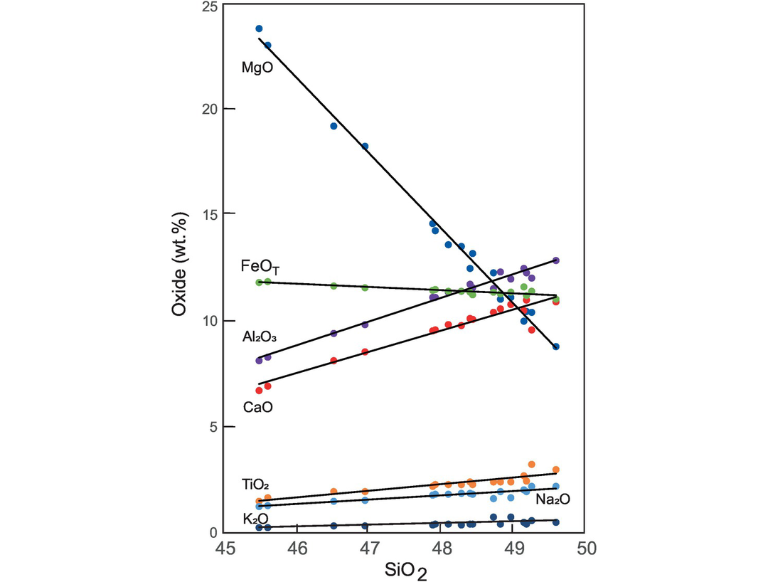
Bivariate plots of major element oxides versus SiO2. The data represent basaltic lavas from the lava lake Kīlauea Iki associated with the 1959–1960 volcanic eruption of Kīlauea, Hawai‘i (from Richter and Moore, 1966). A linear trend is fitted for each of the oxides. The data are given in Table 3.6.
3.3.1 Recognising Geochemical Processes on a Major Element Variation Diagram
Most trends on variation diagrams are the result of mixing. In igneous rocks the mixing may be between two magmas, because of the addition and/or subtraction of solid phases during contamination or fractional crystallisation, or due to the addition of melt increments during partial melting. In sedimentary rocks trends on a variation diagram will also result from mixing, but in this case it is the mixing of chemically distinct components that defines the composition of the sediment. In metamorphic rocks trends on a variation diagram will usually reflect the processes in the igneous or sedimentary protolith, masked to some degree by specific metamorphic processes such as metasomatism, the chemical alteration of a rock by non-deuteric fluids. In some instances, however, deformation can mechanically mix more than one rock type, giving rise to a mixing line of metamorphic origin. Below we consider some of the more important mixing processes.
3.3.1.1 Fractional Crystallisation
Fractional crystallisation is a major process in the evolution of many igneous rocks and is frequently the cause of trends seen on their variation diagrams. The fractionating mineral assemblage is normally indicated by the phenocrysts present. A test of crystal fractionation may be made by accurately determining the composition of the phenocrysts using an electron microprobe and then plotting the compositions on the same graph as the rock analyses. If trends on a variation diagram are controlled by phenocryst compositions, it may be possible to infer that the rock chemistry is controlled by crystal fractionation. It should be noted, however, that (1) fractional crystallisation may take place at depth in which case the fractionating phases may not be represented in the lower pressure and temperature phenocryst assemblage and, as discussed below, that (2) mineralogical control can also be exercised by partial melting processes.
The importance of fractional crystallisation was expounded at length by Bowen (1928) in his book The Evolution of the Igneous Rocks and who argued that geochemical trends for volcanic rocks represent a ‘liquid line of descent’. This is the path taken by residual liquids as they evolve through the differential withdrawal of minerals from the magma. The ideas of Bowen now need to be qualified in the context of modern findings in the following ways:
1. Trends identical to those produced by crystal fractionation can also be produced by partial melting.
2. Only phenocryst-poor or aphyric volcanic rocks will give a true indication of the liquid path.
3. Rarely does a suite of volcanic rocks showing a progressive chemical change erupt in a time sequence. Even a highly correlated trend on a variation diagram of phenocryst-free volcanic rocks from a single volcano is unlikely to represent a liquid line of descent. Rather, it represents an approximation of the liquid line of descent of similar, overlapping, sub-parallel lines of descent.
As an example, the variation in composition of olivine-rich basalts from the lava lake Kīlauea Iki, Hawai‘i (Table 3.6), are presented as bivariate plots (Figure 3.12). This variation is thought to be the product of fractional crystallisation which was ‘controlled principally by the physical addition or removal of olivine phenocrysts’ (Richter and Moore, 1966). A detailed comparison with olivine compositions indicates that other phases were also involved in crystal fractionation but that olivine was the major control.
3.3.1.2 Assimilation and Fractional Crystallisation
If phenocryst compositions cannot explain trends in a rock series and a fractional crystallisation model does not appear to work, it is instructive to consider the possibility of simultaneous processes such as assimilation of the country rock combined with fractional crystallisation. Assimilation plus fractional crystallisation, often abbreviated AFC, was first proposed by Bowen (1928), who argued that the latent heat of crystallisation during fractional crystallisation can provide sufficient thermal energy to consume the wall rock. Consequently, hot magmas undergoing fractional crystallisation assimilate cool crust as a consequence of heat transfer from the magma to the crust.
Kuritani et al. (2005) illustrate this process for an alkali basalt-dacite suite from the magma chamber of the Rishiri volcano in northern Japan. They show that major element variations in the lava suite can be explained by mixing of a magma in the main magma body with a melt transported from a mushy boundary layer in the partially fused floor of the magma chamber. A slightly different example comes from mantle petrology where very high temperature melts have the capacity to react with the rock through which they are transiting, in particular, when the two are out of equilibrium. A well-studied example is the reaction between MORB melts and highly depleted harzburgitic mantle. This reaction consumes orthopyroxene and precipitates olivine, leading to dunite channels in the harzburgite which indicate the route followed by the migrating melt (e.g., Kelemen, 1990 and Kelemen et al., 1995).
It has been proposed that AFC processes can result in the ‘decoupling’ of the major element chemistry from that of the trace elements and/or isotopes and so may not always be evident in the major element data. For example, the contamination of a basalt precipitating olivine, clinopyroxene and plagioclase will result in increased precipitation of the fractionating minerals but may cause only a minor change in the silica content of the liquid. Trace element levels and isotope ratios, however, might be changed and provide a better means of recognising assimilation.
3.3.1.3 Partial Melting
Progressive fractional melting will show a trend on a variation diagram which is controlled by the chemistry of the solid phases being added to the melt. However, this can be very difficult to distinguish from a fractional crystallisation trend on a major element variation diagram, for both processes represent crystal–liquid equilibria involving almost identical liquids and identical minerals. One way in which progressive partial melting and fractional crystallisation may be distinguished using major elements is if the two processes take place under different physical conditions. For example, if partial melting takes place at great depth in the mantle and fractional crystallisation is a crustal phenomenon, then some of the phases involved in partial melting will be different from those involved in fractional crystallisation. Trace elements (discussed in Chapter 4) provide additional means of discriminating between these two processes.
3.3.1.4 Mixing Lines in Sedimentary Rocks
Trends on variation diagrams for sedimentary rocks may result from the mixing of the different components which constitute the sediment. There are a number of examples of this effect in the literature. Bhatia (1983) in a study of turbidite sandstones from eastern Australia presented bivariate plots (Figure 3.13) in which there is a change in the mineralogical maturity, as evidenced by an increase in quartz (SiO2) coupled with a decrease in the proportions of lithic fragments and feldspar represented by the other oxides.
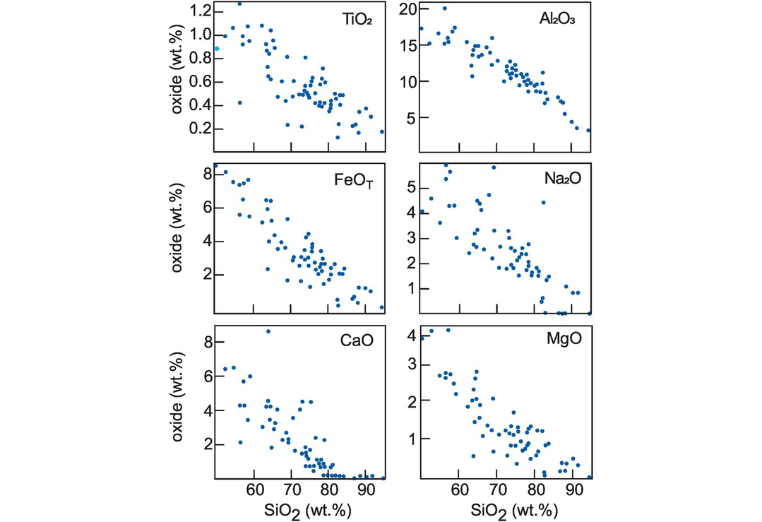
Bivariate plots for quartz-rich sandstone suites from eastern Australia (after Bhatia, 1983). The increase in SiO2 reflects an increased mineralogical maturity, that is, a greater quartz content and a smaller proportion of other detrital minerals.
3.3.1.5 The Identification of Former Weathering Conditions in Sedimentary Rocks
A good measure of the degree of chemical weathering can be obtained from the chemical index of alteration (CIA; Nesbitt and Young, 1982):
Concentrations are expressed as molar values and CaO* is CaO in silicate phases only. The index was originally devised to reconstruct palaeoclimatic conditions from early Proterozoic sediments in northern Canada but has subsequently been used as a proxy to quantify the intensity of chemical weathering in drainage basins (Shao et al., 2012).
An extension of the CIA index is the (CaO* + Na2O)–Al2O3–K2O triangular plot (Nesbitt and Young (1984, 1989). On a diagram of this type the initial stages of weathering form a trend parallel to the tie between (CaO* + Na2O) and Al2O3 of the diagram, whereas advanced weathering shows a marked loss in K2O as compositions move towards the Al2O3 apex (Figure 3.14a). The trends follow mixing lines representing the removal of alkalis and in solution the breakdown of first plagioclase and then potassium feldspar and finally the ferromagnesian silicates. Deviations from such trends can be used to infer chemical changes resulting from diagenesis or metasomatism (Nesbitt and Young, 1984, 1989). This approach has also been applied to mudstones, and the major and trace element chemistry of ancient and modern muds can be used to determine the degree of weathering in their source (Nesbitt et al., 1990).
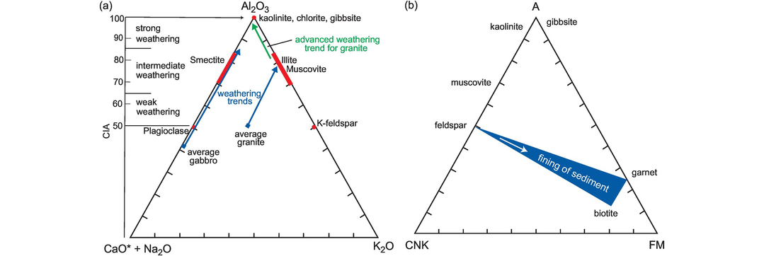
Weathering effects. (a) The (CaO + Na2O)–Al2O3–K2O diagram showing weathering intensity and the weathering trends for an average granite and an average gabbro (after Nesbitt and Young, 1984, 1989; Shao et al., 2012). The advanced weathering trend for granite is also shown. Compositions are plotted as molar proportions. CaO* represents the CaO associated with the silicate fraction of the sample. (b) The A (Al2O3), CNK (CaO + Na2O + K2O), FM (FeOT + MgO) molar proportions diagram showing chemical change with sediment grain size.
Nesbitt and Young (1996) also proposed an A–CNK–FM diagram which uses the molar proportions of Al2O3–(CaO + Na2O + K2O)–(FeOT + MgO) to show those chemical changes in sediments which are a function of grain size. It also demonstrates an increase in the ferromagnesian component with decreasing grain size (Figure 3.14b).
3.3.1.6 Artificial Trends
Sometimes trends on variation diagrams are artificially produced by the numerical processes used in plotting the data rather than reflecting geochemical relationships. This is well documented by Chayes (1960) and Aitchison (1986), who have shown that correlations in compositional data can be forced as a result of the unit sum constraint (see Section 2.2). The most helpful way to circumvent this problem is to examine trends on variation diagrams in the light of a specific hypothesis to be tested. The closeness of fit between the model and the data can then be used to evaluate the hypothesis.
3.3.2 Selecting a Variation Diagram
Two main types of variation diagrams – bivariate plots and ternary diagrams – are widely used by geochemists and are considered here.
3.3.2.1 Bivariate Plots
The principal aim of a bivariate plot, such as that illustrated in Figure 3.12, is to show variation between samples and to identify trends. Hence the element plotted along the x-axis of the diagram should be selected either to show the maximum variability between samples or to illustrate a particular geochemical process. Normally, the oxide which shows the greatest range in the dataset would be selected – in many cases this would be SiO2, but with basic igneous rocks it could be MgO and in clay-bearing sediments Al2O3. The initial stage of a geochemical investigation often requires the preparation of a large number of diagrams in order to delimit the possible geological processes operating. In such cases the initial screening of the data is best done using a correlation matrix (see Section 2.4.5) to explore for strong correlations. However, it is important to remember that meaningless correlations can arise through a cluster of data points and a single outlier. Similarly, poor correlations can arise if the dataset contains multiple populations, each with a different trend. More normally, and more fruitfully, most geochemical investigations are designed to solve a specific problem and to test a particular hypothesis – usually formulated from geological or other geochemical data. In this case the plotting parameter for a variation diagram should be selected with the process to be tested in mind. For example, in the case of an igneous rock suite for which a crystal fractionation mechanism is envisaged, then an element should be selected which is contained in the fractionating phase and that will be enriched or depleted in the melt.
(a) Bivariate plots using SiO2 as the x-axis. These are the oldest form of variation diagram and are one of the most frequently used means of displaying major element data (see Figures 3.12 and 3.13). SiO2 is commonly chosen as the plotting parameter for many igneous rock series and for suites of sedimentary rocks with a variable quartz content because it is the major constituent of the rock and shows greater variability than any of the other oxides. However, the very fact that SiO2 is the most abundant oxide can sometimes lead to spurious correlations, as discussed in Section 3.3.2.2.
(b) Bivariate plots which use MgO as the x-axis. Another common bivariate diagram uses MgO on the x-axis instead of SiO2. This is most appropriate for mafic and ultramafic suites in which the range of SiO2 concentration may be small. MgO, on the other hand, is an important component of the solid phases in equilibrium with mafic melts, such as olivine and the pyroxenes, and shows a great deal of variation due either to the breakdown of magnesian phases during partial melting or to their removal during fractional crystallisation. Figure 3.15 shows an olivine-controlled fractionation trend in komatiites from the Belingwe greenstone belt in Zimbabwe (data from Bickle et al., 1993). Mg# (for definition, see subsection (e) below) is sometimes substituted for MgO, but the underlying principle is the same – to use the component with the greatest spread.
(c) Bivariate plots using cations. It is sometimes simpler to display mineral compositions on a variation diagram if major element chemical data are plotted as cation %, that is, the wt.% oxide value divided by the molecular weight and multiplied by the number of cations in the oxide formula and then recast to 100% (see Section 3.2.2 and Table 3.3). Alternatively, the results may be expressed as mol %, that is, the wt.% oxide values divided by the molecular weight and recast to 100% (see Section 3.2.2 and Table 3.3).
(d) Elemental weight ratio plots. The Al/Si versus Mg/Si diagram is used to show differences in the composition of meteoritic materials and identify the processes operating during the differentiation of the Earth’s mantle. These elements are chosen because they represent the more refractory elements formed during the condensation of the solar nebula, and the ratio plot represents the relative fractionation of the different planetary materials. The plotting parameters are calculated by reducing the oxide wt.% of each of the components to their elemental wt.% concentrations; that is, multiply Al2O3 by 0.529, SiO2 by 0.467, and MgO by 0.603. In Figure 3.16 trends for mantle peridotites and meteorites are plotted together with the field for the likely chondritic material parental to the Earth and the primitive mantle compositions from Table 3.2.
(e) Bivariate plots using the magnesium number (Mg#). The older geochemical literature carries a large number of examples of complex, multi-element plotting parameters which were used as a measure of fractionation during the evolution of an igneous sequence. These are rather complicated to use and difficult to interpret, and have fallen into disuse. One which is usefuland so survives, however, is based on the magnesium–iron ratio, the so-called magnesium number. The magnesium–iron ratio is particularly useful as an index of crystal fractionation in basaltic liquids for here the Mg-Fe ratio changes markedly in the early stages of crystallisation as a result of the higher Mg-Fe ratio of the liquidus ferromagnesian minerals than that of their host melts. The Mg# has been variously defined as follows: MgO/(MgO + FeO + Fe2O3), 100 Mg/(Mg + Fe2+), (Mg/Mg + Fetot), and presented either by weight or atomic proportions. We define the Mg# as 100 × Mg2+/(Mg2+ + Fe2+tot) calculated in atomic proportions. To calculate the Mg# divide the wt.% oxide values for MgO and FeOT (recalculated as Fe2+) by their respective molecular weights of 40.3 and 71.8. Whenever the term Mg# is used, the formula used should be specified.
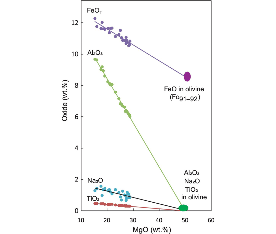
Oxides versus MgO variation for komatiites from the Archaean Belingwe greenstone belt in Zimbabwe (data from Bickle et al., 1993). The extended lines show that the fractionation trend is principally controlled by olivine with the composition Fo91–92. The slight scatter in the Na2O trend probably indicates a small amount of element mobility.
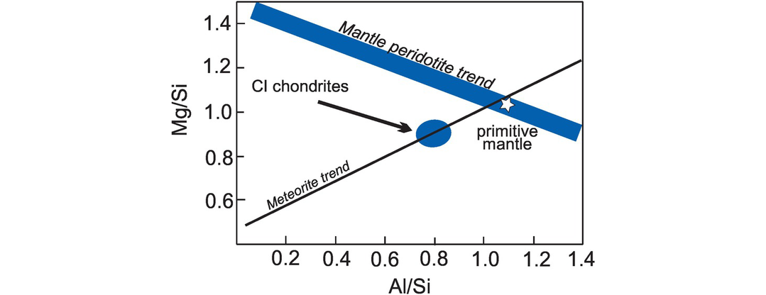
Differentiation of planetary materials. Elemental Al/Si versus Mg/Si plot showing the meteorite and peridotitic mantle trends relative to CI chondrites and the composition of the Earth’s primitive mantle.
3.3.2.2 Compositional Data and Bivariate Diagrams
Statisticians have been warning geochemists about their inappropriate treatment of compositional data for several decades (Section 2.2.2.1). This criticism is typified in the comment on bivariate diagrams by Aitchison and Egozcue (2005), who state that Harker diagrams are ‘best condemned as misleading and best left out of any attempts to interpret compositional variability’. A similar sentiment is put more mildly by Buccianti and Grunsky (2014): ‘Compositional data analysis in geochemistry: Are we sure to see what really occurs during natural processes?’ This ongoing challenge to the time-honoured treatment of compositional data, and in particular, its representation on bivariate plots, presents the geochemical community with a dilemma, but experience seems to suggest that the challenge from the statistical community is misplaced for several reasons:
1. Bivariate diagrams seem to work and yield geologically meaningful results.
2. There is little evidence from the application of the log-ratio approach, the recommended alternative (Section 2.7.1), that this methodology provides a deeper or superior understanding of geochemical and petrological processes as displayed in bivariate plots. This may in part reflect its dominant application to the compositional analysis of soils, volcanic gases and water chemistry (see Buccianti et al., 2006), rather than the geochemical data associated with geochemistry and petrology.
3.3.2.3 So Why Do Bivariate Plots Appear to Work?
An essential element missing from the debate between statisticians and geochemists over the use and misuse of bivariate diagrams is an appreciation of the geological context. When a suite of samples is collected to test a particular hypothesis or to investigate a particular process, the data are set in a particular context which in turn places constraints on the interpretation of the data. In other words – and this is a theme which will recur throughout this text – geological field control is essential for the meaningful interpretation of geochemical data.
Cortés (2009) takes issue with the criticism of bivariate diagrams by Aitchison and Egozcue (2005) and argues that bivariate diagrams ‘are not a correlation tool but [rather] a graphical representation of the mass actions and mass balances in the context of a geological system’. They serve as a simple display of evolutionary trends which are thought to represent a process or set of processes; the trends observed, ‘spurious or not, are given by the law of mass action’. Hence the expectation is not to discover the covariance structure associated with these trends, but rather to interpret them within a geological context, and where trends are observed these may be used as robust evidence of the link between samples. He further argues that trends on bivariate diagrams can be used quantitatively to calculate the proportion of species involved in a particular geological process. For example, he suggests that a suite of basalts from a particular lava flow might be collected because they are expected to be chemically related. If, in addition, there is field evidence to suggest that these basalts have experienced a common process such as olivine fractionation, then there is a testable hypothesis as to the nature of their relationship. Thus, Cortés (2009), following Rollinson (1992), cites the major element oxide data for samples from the Kīlauea Iki lava lake (Table 3.6, Figure 3.12) which show near perfect, but allegedly spurious, correlations. In line with the geological context, however, the trends confirm a common magmatic origin – the working hypothesis behind the data collection. Further, in the context of mass balance, the variation between samples can be shown to be consistent with olivine addition and removal, again the working hypothesis set by the geological context.
We support the logic of Cortés (2009) and argue that given a geological context, bivariate plots can be an important exploratory tool for the visualisation of geochemical data, a point which is also acknowledged by Egozcue (2009) in his response to Cortés’s (2009) critique. Thus, a suite of bivariate plots for a single dataset remains a powerful tool for understanding geological processes. This conclusion is entirely consistent with the view of log-ratios expressed by Rock (1989). Geochemists work with rock compositions in which, for the most part, variation is controlled by minerals with fixed stoichiometries and together these data must be interpreted within the geological context in which the samples were found.
The preceding discussion argues that compositional data analysis may tell us that the correlation coefficient computed for a particular trend is not meaningful and that the correlation is spurious; nevertheless, the trend may be real and have geological meaning. In the case of bivariate major element plots, it is not the value of the correlation coefficient that is important; rather, it is the presence and shape (linear, curvilinear or kinked) of the trends that are significant. These are the properties that need to be interpreted.
3.3.3 Ternary Diagrams
Ternary diagrams, also known as triangular or trivariate diagrams or plots, are used when it is necessary to show simultaneous change between three variables. There are statistical problems associated with the plotting of data on ternary diagrams (Section 2.9) and they must be used with care. The plotting procedure for ternary diagrams is described in Figure 3.17. This can be carried out using an Excel macro that projects orthogonal coordinates onto triangular geometry. These include the free online ‘Triangular Graph Constructor’, ‘Ternary Plot Generator’, or TRI-PLOT (Graham and Midgley, 2000).
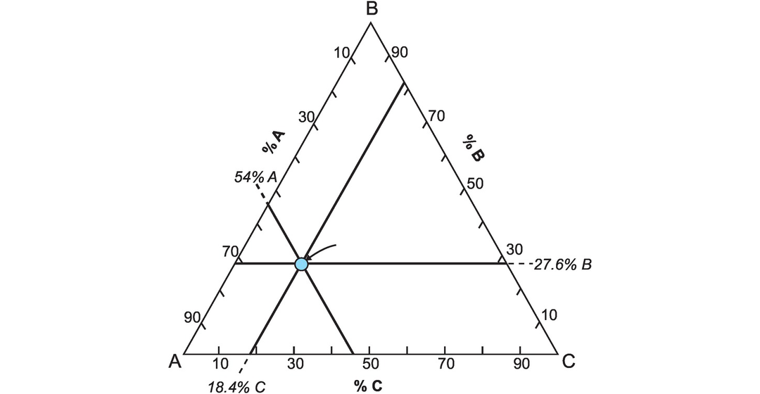
The plotting procedure for triangular diagrams. To plot a single point for the variables A = 54%, B = 27.6% and C = 18.4% on a triangular diagram, follow this procedure. Variable B is 100% at the top of the plotting triangle and 0% along the base of the triangle. Counting upwards from the base (the concentrations are given on the right-hand side of the triangle), draw the horizontal line representing 27.6%. In a similar way draw the line representing A = 54% parallel to the right side of the triangle. The point at which the two lines intersect is the plotting position. To check that it has been accurately located, the line for variable C at 18.4% should pass through the intersection of the two other lines.
3.3.3.1 The AFM Diagram
The igneous AFM diagram (not to be confused with the metamorphic diagram of the same name) is used to distinguish between the tholeiitic and calc-alkaline differentiation trends of the sub-alkaline magma series (Figure 3.18). The diagram takes its name from the oxides plotted at its apices: Alkalis (Na2O + K2O), FeOT and MgO. The plotting parameters are calculated by summing the oxides (Na2O + K2O), (FeO + Fe2O3) recalculated as FeO, and MgO; each component is then recalculated as a percentage of the total. Historically, ambiguity exists over the treatment of Fe, but the standard today is that F should reflect all Fe as FeOT to accommodate most modern analytical data for which the separate oxidation states of iron have not been determined.
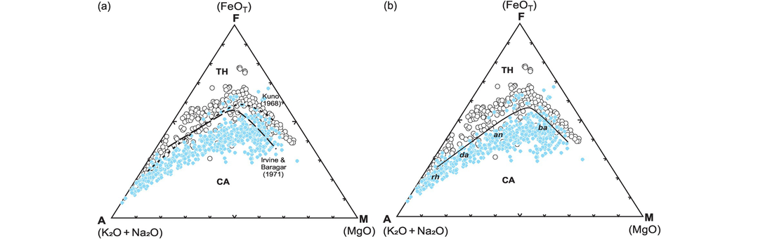
The AFM diagram. This diagram distinguishes between the calc-alkaline (CA) and tholeiitic (TH) rock series. The data points shown represent ∼ 1100 analyses (~500 tholeiitic Icelandic lavas = filled symbols; ~ 600 calc-alkaline Cascade lavas from the western United States = open symbols) taken from www.earthchem.org/portal (NAVDAT and USGS databases). All Fe was converted to FeOT. Only complete analyses with reported locations, low LOIs (< 3 wt.%), and appropriate Na2O + K2O (to exclude alkaline rocks) were used. The data shown here were randomly selected from the filtered dataset and plotted using Tri-plot (Graham and Midgley, 2000). (a) The boundaries of Irvine and Baragar (1971) and Kuno (1968). (b) The new boundary curve recommended here. The coordinates for the curve are A, F, M: 11, 39, 50; 14, 50, 36; 18, 56, 26; 28, 52, 20; 40, 45, 15; 70, 26, 4). ba, basalt; an, andesite; da, dacite; rh, rhyolite.
Most authors use oxide wt.% data when plotting an AFM diagram, but in some cases atomic proportions are used. Since data points plot in different positions depending upon the calculation method (Barker, 1978), it essential to specify which method has been adopted.
The boundary between the calc-alkaline and the tholeiite series on the AFM diagram has previously been defined by Kuno (1968) and Irvine and Baragar (1971) (Figure 3.18a). Both authors use wt.% oxide and represent F as FeOT. Kuno’s boundary defines a smaller field for the tholeiitic suite than that of Irvine and Baragar (Figure 3.18a). Here we define a new boundary curve which better discriminates between the two magma series. We have used representative data for tholeiitic and calc-alkaline lavas from Icelandic lavas and lavas from the Cascades of the western United States, respectively. Our result is shown in Figure 3.18b, and the coordinates for the new curve and details of the analyses used are described in the figure caption.
It is important to note that the AFM diagram is limited in the extent to which quantitative petrogenetic information may be extracted. This is a function of the way in which ternary plots are constructed, for they use percentage data, not absolute values, and use only a part of the rock chemistry. In most rocks the A–F–M components make up less than 50% of the total oxide weight percentage and they are therefore a sub-composition of the rock chemistry. In addition, when a compositionally varied rock series is plotted, different proportions of each sample are normalised to 100%, and so the relationship between the plotted values is distorted. For example, in a series of volcanic rocks in the compositional range basalt to dacite about 40% of the basalt major element chemistry is used when plotting onto an AFM diagram, whereas only about 15% of the dacite major element chemistry is used. For these reasons, the main use of AFM diagrams is to subdivide the sub-alkaline rock series into tholeiitic and calc-alkaline magma types as discussed above.
3.3.4 Interpreting Trends on Variation Diagrams
From the discussion above of bivariate and trivariate plots, it is clear that there are a variety of processes which can produce similar looking trends on major element variation diagrams. It is important therefore to discover the extent to which these various processes might be distinguished from one another and identified.
3.3.4.1 Extract Calculations
One approach is to try to calculate the composition of the materials added to or subtracted from a magma and to quantify the amount of material involved. This may be done using an extract calculation, a method described in some detail by Cox et al. (1979). The method is illustrated in Figure 3.19a in which the chemical compositions (expressed in terms of variables A and B) of both minerals and rocks are plotted on the same variation diagram. Mineral X crystallises from liquid L1 and the residual liquid follows the path to L2. The distance from L1 to L2 will depend upon the amount of crystallisation of mineral X. This may be quantified as follows:
Therefore,
This relationship is known as the lever rule.
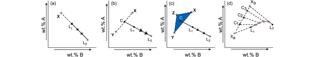
Mineral extract calculations. (a) Mineral X is removed from liquid L1 and the liquid composition moves from L1 to L2; (b) mineral extract C (made up of minerals X and Y) is removed from liquid L1 and drives the liquid composition to L2; (c) mineral extract C (made up of the minerals X, Y and Z) is removed from liquid L1 and drives the resultant liquid composition to L2; (d) mineral X is a solid solution made up of components Xa and Xb. As the mineral composition changes from Xa to Xb via the intermediate compositions C1 to C3 the mineral extracts incrementally change the composition of the liquid from L1 to L2 along a curved path.
If there are two or more minerals crystallising simultaneously from liquid L1 in such proportions that their average composition is C (Figure 3.19b, c), then the liquid path will move from C towards L2. The proportion of solid to liquid will be given by the ratio L1L2:CL1. The proportions of the minerals X and Y in Figure 3.19b is given by YC:XC. In these variation diagrams the predicted trends form straight lines. However, minerals whose compositions vary because of solid solution will produce curved trends during fractionation (Figure 3.19d).
It is also possible to use extract diagrams to seek to understand partial melting processes. However, in practice extract calculations are inexact for often the minerals involved have complex solid solutions. In addition there may be statistical uncertainties in fitting a straight line through the trend on a variation diagram (Cox et al., 1979). For these reasons the differences between mineral melt equilibria in melting reactions and during fractional crystallisation may be difficult to resolve.
3.3.4.2 Addition–Subtraction Diagrams
An alternative approach to identifying the composition of the solid phase during magmatic fractionation is to use an addition–subtraction diagram to calculate the composition of the fractionating phase or phases. In this case the entire major element chemistry of two or more rocks is used and plotted on a bivariate diagram as is shown in Figure 3.20. Back projection of the data shows that five of the elements reduce to zero at 41.5% SiO2, consistent with olivine control. The composition of the olivine can be estimated from the diagram, and a simple calculation shows that composition A can be converted to composition B by the removal of 15% olivine. This result would be confirmed from the presence of olivine phenocrysts in the lava.
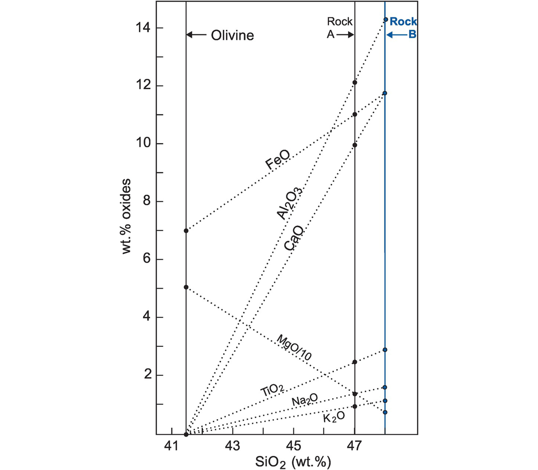
The addition–subtraction diagram for the calculation of the composition of the fractionating phase in magmatic rocks. Using samples A and B it can be shown that rock composition B is generated by the extraction of olivine from the composition of rock A. This is done using the back projection of trends for Al2O3, CaO, TiO2, Na2O and K2O. These converge on zero at SiO2 = 41.5 wt.%, indicating an olivine extract. MgO and FeO values at 41.5 wt.% SiO2 indicate the composition of the olivine removed from rock A to produce composition B.
3.3.4.3 Limitations to the Application of Extract Calculations
In some volcanic rocks it may be difficult to perform an extract calculation because of the large number of phenocryst phases involved. For example, some evolved calc-alkaline lavas may have undergone fractionation of the total assemblage olivine-clinopyroxene-biotite-plagioclase-potassium feldspar-sphene-apatite-magnetite in a series of magma chambers prior to eruption. A further complication is that the close chemical equivalence of mineral assemblages such as plagioclase + olivine, orthopyroxene + augite + magnetite and hornblende can give rise to some ambiguity of interpretation (Gill, 1981).
Other limitations to extract calculations are when the observed liquid line of descent is in reality a mix of several lines, when the compositions of the crystallising phases change during the process of fractionation with the changing composition of the magma and when the phenocrysts present in lava are not representative of the fractionating phases.
3.3.4.4 Trends Showing an Inflection
Some variation diagrams are segmented and show an inflection point. The inflection generally indicates either the entry of a new phase during crystal fractionation or the loss of a phase during partial melting. This is illustrated with the data of Garcia et al. (2018) for basaltic glasses from the Keanakāko‘i Tephra from Kīlauea, Hawai‘i (Figure 3.21). Data plotted on MgO variation diagrams for the oxides CaO, FeOT, Al2O3, and K2O show that at ≥7 wt.% MgO, CaO and Al2O3 increase as MgO decreases, whereas below 7 wt.% MgO the oxide concentrations of CaO and Al2O3 decrease and FeOT and K2O increase. These trends suggest that at MgO concentrations ≥7 wt.% the changing melt compositions are controlled by olivine fractionation during which MgO is removed from the melt and the relative proportions of residual CaO and Al2O3 increase. At MgO concentrations <7 wt.% the co-precipitation of plagioclase and clinopyroxene reduce the absolute amount of CaO and Al2O3 in the melt and the relative proportions of FeOT and K2O increase due to the constant sum effect (Section 2.2.2.1).
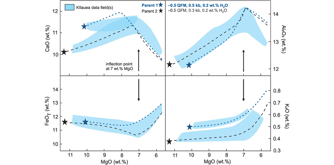
Select bivariate plots for the Keanakāko‘i Tephra from Kīlauea, Hawai‘i (after Garcia et al., 2018). Shaded regions represent the data fields. The change in slope at about MgO = 7 wt.% in CaO, Al2O3, FeOT and K2O is consistent with a change in the fractionating phases at this point. The two dashed lines represent the best-fit forward modelling compositional trends using AlphaMELTS (Smith and Asimow, 2005) which indicate that the range in tephra composition is consistent with crystal fractionation at low pressure (0.3–0.5 kb), low water content (0.2 wt.% H2O) and an oxygen fugacity of QFM = −0.5.
Inflections will be apparent on variation diagrams of a rock series only if the chemistry of the extracted phase is reflected in the plotting parameters. However, when inflections are present they should be located at the same point in the rock series as is the case for the Hawaiian data shown in Figure 3.21. Inflections are most obvious when the number of fractionating minerals is small as in basaltic melts. In calc-alkaline volcanic rocks, where the number of fractionating phases is large, the entry or exit of a single phase may not sufficiently affect the bulk chemistry of the melt to be seen on a variation diagram.
3.3.4.5 Scattered Trends
Observation shows that some variation diagrams define well-constrained trends whereas others do not. For example, the data for Kīlauea Iki illustrated in Figure 3.12 show very clear trends which are indicative of one main geological process. In contrast the data for the Australian sandstones illustrated in Figure 3.13 shows more scattered trends, as do some of the trends in the data for the Limpopo Belt tonalitic and trondhjemitic gneisses listed in Table 2.2.
In general terms, scattered trends on variation diagrams may arise through the following:
Sampling error: For example, samples may have been collected over a wide area but they are not all genetically related. Alternatively, an unintended bias may be present in the sampling process.
Analytical error: Scatter on variation diagrams can arise through uncertainties in the analytical measurements or when measurements on subsets of the data have been made in different laboratories.
The operation of multiple geological processes: In the case of the data for the Belingwe Greenstone Belt (Figure 3.15) the greater scatter associated with Na2O versus MgO might indicate a primary control by olivine fractionation combined with secondary scatter due to Na mobility related to late fluid movement through the rock.
In sedimentary rocks scatter may be a function of the mixing processes leading to the formation of the sediment.
In metamorphic rocks scattered trends may reflect the geochemical imprint of a metamorphic process on earlier igneous or sedimentary processes.
In igneous rocks a scattered trend can arise for a number of reasons: these include the mixing of melt and cumulus minerals due to either the accumulation of phenocrysts in a lava or the formation of a cumulate rock in a magma chamber, the sampling of multiple magma compositions in a lava pile, and/or a change in the fractionating assemblage during fractional crystallisation.
3.3.5 Modelling Major Element Processes in Igneous Rocks
Computer-based modelling offers a quantitative alternative to the deductive use of variation diagrams for investigating petrological processes. There are two approaches. Forward modelling begins with a known starting composition and determines how this composition will evolve to a derivative or daughter composition given specific physical conditions. Inverse modelling begins with a derived composition and works ‘backwards’ to determine the composition of the parent. If both starting and end compositions are known, as for example in a volcanic series, it is possible to explore the processes that might link the two. These might include the addition or removal of mineral phases, changes in pressure and temperature during the evolution of the magma, and/or the amount of H2O present in the melt. Models of this type are designed to use real analytical data in order to test specific hypotheses regarding magma genesis and they provide feasible but not necessarily unique pathways of magma evolution. If a rock has a complex history, the modelling may be better formulated as a series of steps.
The success of any model is estimated from the residuals of the calculation, that is, the difference between the actual and calculated compositions (Table 3.7). In addition all model results should be evaluated petrologically and the relative proportions and composition of the calculated fractionating phases should be compared with the phenocryst assemblage present in the sample suite. A computer model will normally produce a ‘best-fit’ solution, although it is important to stress that the result may be non-unique and that the ‘solution’ is not always correct. For this reason, many workers test models based on major element chemistry with further calculations based upon trace element and/or isotopic data.
3.3.5.1 Modelling Fractional Crystallisation
In their simplest forms, fractional crystallisation models take the general form
This generalised equation can be rearranged to solve for any of the parameters involved such as the parent melt, the derived melt or the crystallising assemblage. For a given silicate liquid, the aim of the modelling is to determine the nature of crystallising phase, the composition of the melt at the different stages during its evolution, the temperature of crystallisation, and the crystallisation sequence of the phases. Three different approaches are used:
1. The calculation of the distribution of major elements between mineral phases and a coexisting silicate melt from experimental phase equilibria using regression techniques.
2. The determination of mineral–melt equilibria from measured distribution coefficients.
3. The application of equilibrium thermodynamic models for magmatic systems. These require valid mixing models for the liquid and an internally consistent set of solid–liquid thermochemical data.
Wright and Marsh (2016) performed fractional crystallisation calculations (Table 3.7) for Kīlauea volcano, Hawai‘i, using a least squares regression technique. The purpose of the study was to test whether or not the more differentiated lavas erupted from Kīlauea’s East Rift Zone were derived from the more primitive compositions from the Kīlauea caldera summit more than 30 km to the west. Using the oxide compositions of phenocrysts combined with whole rock compositions and the temperature of the presumed parents, they were able to determine the percentages of olivine, augite, plagioclase and ilmenite necessary to generate the differentiated lavas from the assumed parent composition. The very low values calculated for the maximum and minimum residuals in Table 3.7 confirm the reasonableness of the results.
| Parent | Differentiate | Minerals removed from parent | Residuals | |||||||||
|---|---|---|---|---|---|---|---|---|---|---|---|---|
| Olivine | Augite | Plagioclase | Ilmenite | Max. | Min. | |||||||
| 1955 components | 1921 | 1955E, MgO = 5.39 | 3.00 | 22.42 | 21.84 | 1.66 | ||||||
| Composition (wt.%) | 100 | 51.08 | Fo70 | An61 | 0.005 | 0.00 | ||||||
| 1977 components | 1961 | 1977, MgO = 5.34 | 3.85 | 17.31 | 15.29 | 0.58 | ||||||
| Composition (wt.%) | 100 | 62.97 | Fo77.1 | An68.4 | 0.006 | 0.001 | ||||||
| 1977 components | 1961 | 1977, MgO = 5.89 | 3.20 | 12.80 | 10.31 | 0.29 | ||||||
| Composition (wt.%) | 100 | 73.39 | Fo77.1 | An69.38 | 0.01 | 0.001 | ||||||
The thermodynamic modelling of phase equilibria offers a powerful approach for investigating processes in magmatic systems. Of the software packages available, the MELTS (http://melts.ofm-research.org) suite of programs is widely used. These programs permit the calculation of equilibrium phase relations for mafic magmatic systems (Ghiorso and Sack, 1995; Asimow and Ghiorso, 1998) and felsic systems (Gualda et al., 2012; Ghiorso and Gualda, 2015) over a broad range of temperatures and pressures (500–2000°C, 0–2 GPa). They are used to explore magmatic processes such as adiabatic decompression melting, energy-constrained assimilation and, post-entrapment crystallization in melt inclusions. They also permit the evaluation of oxygen fugacity in magmatic systems and monitor magmatic evolution along specified oxygen buffers. In addition, it is possible quantify the amount of water present in a magmatic system and model this as a function of temperature, pressure and liquid composition.
Garcia et al. (2018) used AlphaMELTS, the menu-driven interface to subroutines of MELTS (Smith and Asimow, 2005), to constrain the petrogenesis of the Keanakāko‘i Tephra from Kīlauea in Hawai‘i (Figure 3.21). They showed through the forward modelling from inferred parent compositions that the tephra must have formed under conditions of low pressure, low water content and low oxygen fugacity (Figure 3.21). Although the model did not constrain all subsets of the data, it provides a theoretical constraint on the petrogenesis of a significant part of the Keanakāko‘i Tephra.
3.3.5.2 Modelling Fractional Crystallisation and Assimilation
The MELTS software is also incorporated into a comprehensive modelling program known as the Magma Chamber Simulator (MCS) of Bohrson et al. (2014) (https://mcs.geol.ucsb.edu/). The MCS integrates major element, trace element and isotopic data into an energy- and mass-constrained open-system thermodynamic computational tool. It uses energy-constrained assimilation-fractional crystallization equations that account for heating and partial melting of crustal wall rock. Heinonen et al. (2016, 2019) used the MCS to constrain the petrogenesis of Karoo flood basalts from Vestfjella in western Dronning Maud Land, Antarctica. They were able to show that the Vestfjella continental flood basalts could be produced by minor (1–15 wt.%) contamination of asthenospheric parental magmas with lithospheric melts. Their work implies that estimates for the degree of contamination of continental flood basalts by the continental lithosphere are likely to be overestimated (Heinonen et al., 2016).
3.4 Diagrams on Which Rock Chemistry and Experimentally and Thermodynamically Determined Phase Boundaries Are Plotted Together
A number of igneous systems have been sufficiently well determined in the laboratory to allow the geochemist to interpret natural rock compositions in the light of experimentally determined phase boundaries. Increasingly, laboratory data for a system such as mantle peridotite are synthesised from a variety of sources, parameterised, and the results extrapolated using thermodynamic modelling to be widely applicable across a range of melting conditions and source compositions. Diagrams of this type seek to simplify multivariate experimental data sets by projecting the results onto a two-dimensional plane and allowing natural rock data to be projected onto them in a similar manner for interpretive purposes.
Historically, the purpose of many experiments on basaltic and granitic systems was to determine the composition of primary magmas using simplified rock compositions. However, there are problems with this approach for its success depends upon the extent to which the system under investigation matches the natural rock composition; it is now known that presence of only a few percent of an additional component may dramatically change the position of the phase boundaries. Further it is also apparent that some (felsic) rock compositions do not always equate to melt compositions.
In the classical literature the results of multi-oxide experimental studies were projected from a tetrahedron into a planar representation. More recently, the results of experimental studies tend to be expressed in a series of bivariate plots which are simpler to interpret and do not require complex projection procedures. However, there remain a number of projections still in use, and since they are still sometimes referred to, they are described briefly below and summarized in Box 3.2. Each projection is slightly different and has distinct rules. A more general approach to transforming data from quaternary systems into ternary plots is given in the works of Maaloe and Abbott (2005) and Shimura and Kemp (2015).
Melting the mantle
The Yoder–Tilley CIPW normative tetrahedron
The normative Ne-Di-Ol-Hy-Q diagram
Projections in Ol-Pl-Di-Q
The low-pressure tholeiitic phase diagram of Cox et al. (1979)
FeO-MgO plots
Melting mafic crust
Melting felsic (continental) crust
The granite system
Partial melting of crustal rocks
3.4.1 Melting the Mantle
The mineralogy of the upper mantle can be simplified to the phases olivine + orthopyroxene together with minor amounts of clinopyroxene and an aluminous phase (either plagioclase, spinel or garnet depending on pressure). Chemically, the rocks of the mantle simplify to the oxides CaO–MgO–Al2O3–SiO2, often abbreviated to CMAS. Together with Na2O (CMASN) this simplified system also represents the compositional range of most basaltic melts. These mineralogical and chemical systems are the basis for many common projection schemes used to represent mantle melting processes and the evolution of basaltic melts. The most commonly used include the following:
1. The Yoder and Tilley (1962) scheme based upon the main normative minerals observed in basalts (diopside–olivine–anorthite–quartz–nepheline).
2. The CMAS system of O’Hara (1968) based on the oxides CaO–MgO–Al2O3–SiO2 as indicated above.
The two schemes are broadly parallel inasmuch as diopside = C, olivine = M, anorthite = A, quartz = S, and nepheline = Na2O.
3.4.1.1 The Yoder and Tilley CIPW Normative Tetrahedron
The normative nepheline–diopside–olivine–quartz tetrahedron was originally proposed by Yoder and Tilley (1962) for the classification of basalts as illustrated in Figure 3.22a and discussed in Section 3.2. The tetrahedron has also been extensively used for comparing the results of experimental studies on mantle peridotites with the chemical composition of basalts and is the focus of this discussion. A variety of projection procedures have been used and these are outlined below.
(a) The normative Ne–Di–Ol–Hy–Q diagram. This diagram in Figure 3.6 represents the full range of compositions considered in the Yoder and Tilley (1962) tetrahedron (Figure 3.22a) and as previously noted is a means of classifying basalts using their CIPW normative compositions (Thompson, 1984). It can also be used to display experimental and natural rock data for basalts which range from saturated to undersaturated compositions (Thompson, 1984; Gibson et al., 2000) and to show the changing composition of initial melts of different mantle compositions, produced at different pressures (Figure 3.22b).
The calculation procedure is as follows:
CIPW normative compositions are calculated on a wt.% basis and plotted on one of the three triangles.
Fe2O3 is calculated as 15% of the total iron content.
An example of how the diagram may be used is given in Figure 3.22b, which shows the fields of flood basalts and ferro-picrites from the Parana province (Gibson et al., 2000) together with the 1 atm and 9 kb cotectics for melts in equilibrium with olivine, plagioclase and clinopyroxene (data from Thompson, 1983). A variant of the diagram is used by Falloon et al. (2001) in which the Ne-apex is replaced by jadeite + Ca-Tschermak’s + leucite (Jd + CaTs + Lc). In this case molecular norms are projected from olivine onto Di–Qz–Jd + CaTs + Lc and from diopside onto Ol–Qz–Jd + CaTs + Lc.
(b) Projections in the tholeiitic basalt tetrahedron Ol–Pl–Di–Q. A restricted portion of the Yoder and Tilley (1962) diagram – the silica-saturated, tholeiitic basalt segment of the tetrahedron – delimited by the phases olivine–plagioclase–diopside–quartz has also been used extensively for demonstrating relationships between melting experiments and mafic igneous rocks. In this case four different algorithms by Walker et al. (1979), Elthon (1983), Grove (1993) and Presnall et al. (2002) have been devised for plotting experimental and rock data (Figures 3.23 and 3.24). Because the plotting parameters are slightly different from each other, and the allocation of Fe between Fe2+ and Fe3+ also differs, it is important to note which plotting procedure is used in any given projection of the data. An example of each of the calculation schemes is presented in Table 3.8.
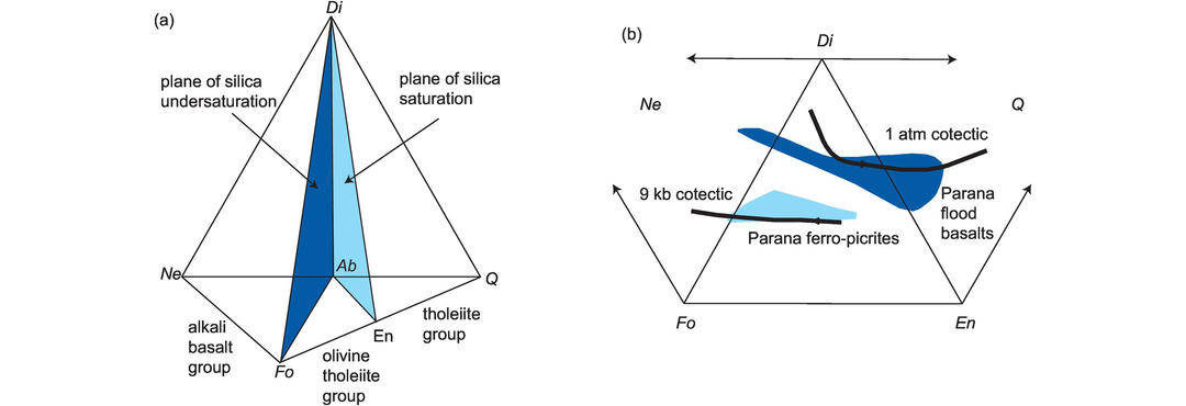
(a) The normative diopside (Di)–nepheline (Ne)–forsterite (Fo)–enstatite (En)–quartz (Q)–albite (Ab) tetrahedron after Yoder and Tilley (1962) showing the diopside–albite–forsterite plane of silica undersaturation, compositions to the left of which contain normative nepheline, and the diopside–albite–enstatite plane of silica saturation, compositions to the right of which contain normative quartz. (b) The planar projection of the Yoder and Tilley tetrahedron showing the expanded Di–Fo–En face and extensions into Ne-normative undersaturated compositions and Q-normative saturated compositions. Also shown are wt.% normative data for ferro-picrites and flood basalts from the Parana province together with low-pressure and high-pressure cotectics for liquids in equilibrium with Ol, Pl, and Cpx from Thompson et al. (1983).
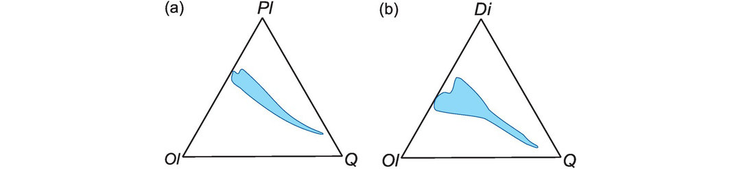
Projections of MORB glass compositions in the tholeiitic basalt tetrahedron Ol–Pl–Di–Q using the molar norm method of Presnall et al. (2002). (a) The diopside projection onto the Pl–Ol–Q plane. (b) The plagioclase projection onto the plane of Di–Ol–Q.
| Wt.% oxide of rock | Mol wt | Mol prop | Mol % | Grove conversion | Grove mol % | |||||
|---|---|---|---|---|---|---|---|---|---|---|
| SiO2 | 50.60 | 60.09 | 0.8421 | 52.92 | 52.92 | 47.19 | ||||
| TiO2 | 1.67 | 79.90 | 0.0209 | 1.31 | 1.31 | 1.17 | ||||
| Al2O3 | 14.79 | 101.96 | 0.1451 | 9.12 | AlO0.5 | 18.23 | 16.26 | |||
| Fe2O3 | 0.00 | 159.69 | 0.0000 | 0.00 | Fe3+ O1.5 | 0.00 | 0.00 | |||
| FeO | 10.46 | 71.85 | 0.1456 | 9.15 | 9.15 | 8.16 | ||||
| MnO | 0.19 | 70.94 | 0.0027 | 0.17 | 0.17 | 0.15 | ||||
| MgO | 7.42 | 40.30 | 0.1841 | 11.57 | 11.57 | 10.32 | ||||
| CaO | 11.38 | 56.08 | 0.2029 | 12.75 | 12.75 | 11.37 | ||||
| Na2O | 2.77 | 61.98 | 0.0447 | 2.81 | NaO0.5 | 5.62 | 5.01 | |||
| K2O | 0.19 | 94.20 | 0.0020 | 0.13 | KO0.5 | 0.25 | 0.23 | |||
| P2O5 | 0.18 | 141.95 | 0.0013 | 0.08 | PO2.5 | 0.16 | 0.14 | |||
| TOTAL | 99.65 | 1.5913 | 100.00 | 112.13 | 100.00 | |||||
| FMO | 18.48 | |||||||||
| Alk | 5.24 | |||||||||
| Plotting procedure of Presnall et al. (2002) | ||||||||||
| Pl = Al2O3–K2O (molecular) | 0.143 | |||||||||
| Di = CaO + K2O + Na2O–3.33P2O5–Al2O3 | 0.100 | |||||||||
| Ol = (MgO + FeO + MnO + 3.33P2O5 + Al2O3–TiO2–Cr2O3–Fe2O3–CaO–K2O–Na2O)/2 | 0.106 | |||||||||
| Q = SiO2–5.5(K2O + Na2O) –0.5(Al2O3 + MgO + FeO + MnO–TiO2–Fe2O3)–1.5CaO + 5P2O5 | 0.059 | |||||||||
| Plagioclase projection | % | |||||||||
| di = | 0.100 | 37.90 | ||||||||
| ol = | 0.106 | 39.87 | ||||||||
| q = | 0.059 | 22.23 | ||||||||
| sum = | 0.265 | 100.00 | ||||||||
| Plotting procedure of Walker et al. (1979) | ||||||||||
| PLAG = Al2O3 + Na2O + K2O(molecular) | 0.192 | |||||||||
| DI = CaO–Al2O3 + Na2O + K2O | 0.105 | |||||||||
| OL = (FeO + MgO + MnO + 2Fe2O3 + Al2O3–CaO–Na2O–K2O)/2 | 0.114 | |||||||||
| SIL = SiO2–(Al2O3 + FeO + MgO + MnO + 3CaO + 11Na2O + 11K2O + 2Fe2O3)/2 | 0.042 | |||||||||
| Plagioclase projection | % | |||||||||
| DI = | 0.105 | 40.14 | ||||||||
| OL = | 0.114 | 43.72 | ||||||||
| SIL = | 0.042 | 16.15 | ||||||||
| sum = | 0.261 | 100.00 | ||||||||
| Plotting procedure of Elthon (1983) | ||||||||||
| PLAG = Al2O3 + Fe2O3 (molecular) | 0.145 | |||||||||
| DI = CaO + Na2O + K2O–Fe2O3–Al2O3 | 0.105 | |||||||||
| OL = ((FeO + MgO + MnO–TiO2) + (Al2O3 + Fe2O3)–(CaO + Na2O + K2O))/2 | 0.103 | |||||||||
| SIL = SiO2–((FeO + MgO + MnO–TiO2) + (Al2O3 + Fe2O3) + 3(CaO + Na2O + K2O))/2 | 0.239 | |||||||||
| Plagioclase projection | % | |||||||||
| Di = | 0.105 | 23.38 | ||||||||
| Ol = | 0.103 | 23.12 | ||||||||
| Si = | 0.239 | 53.50 | ||||||||
| Sum = | 0.447 | 100.00 | ||||||||
| Plotting procedure of Grove et al (1993) | ||||||||||
| Sum = SiO2–CaO–2 × Alk + Cr2O3 + TiO2 (molecular %) | 26.52 | |||||||||
| Qtz = (SiO2–0.5 × FeMO–1.5 × CaO–0.25 × AlO1.5–2.75 × Alk + 0.5 × Cr2O3 + TiO2)/sum | 0.136 | |||||||||
| Plag = 0.5(AlO1.5 + NaO0.5–KO0.5)/(sum) | 0.445 | |||||||||
| Oliv = (FMO + 0.5 × (AlO1.5–Alk)–CaO–TiO2–Cr2O3 + 1.667 × PO2.5)/(2*sum) | 0.194 | |||||||||
| Cpx = (CaO–0.5 × AlO1.5 + 0.5 × Alk–1.667 × PO2.5)/sum | 0.221 | |||||||||
| Plagioclase projection | % | |||||||||
| Cpx = | 0.221 | 40.14 | ||||||||
| Ol = | 0.194 | 35.18 | ||||||||
| Q = | 0.136 | 24.68 | ||||||||
| Total = | 0.551 | 100.00 | ||||||||
Presnall et al. (2002) recalculated rock compositions as CIPW norms, setting the Fe2+/(Fe2+ + Fe3+) ratio to 0.91. The mineral proportions are expressed as mole percent and the plotting parameters are defined as follows:
Hypersthene is calculated as equivalent olivine and quartz. The main projections in the tetrahedron Di–Ol–Pl–Q are from diopside onto the Pl–Ol–Q face, and from plagioclase onto the Di–Ol–Q face. In the case of the plagioclase projection, the proportions of Di, Ol and Q are normalised to their sum and plotted on a molecular basis. The diopside projection is calculated in a similar manner (see Table 3.8). An example of the use of this projection scheme is shown in Figure 3.23, the projection of MORB glass compositions from Di onto the Pl–Ol–Q face and from Pl onto the Di–Ol–Q face of the tholeiitic basalt tetrahedron Ol–Pl–Di–Q (data from Presnall et al., 2002).
Walker et al. (1979) developed a different algorithm for plotting data in the same projections, although the end result is similar to that of Presnall et al. (2002). Weight % oxides are divided by their molecular weight to obtain molecular proportions, all Fe is presented as FeO, and the plotting parameters are calculated from the molecular proportions as follows:
Walker et al. (1979) use the notation DI–OL–SIL and OL–SIL–PLAG for projections from plagioclase onto the Di–Ol–Q face and from diopside onto the Pl–Ol–Q face. In the case of the plagioclase projection. the proportions of DI, OL and SIL are calculated and then normalised to their sum (Table 3.8) and plotted on a molecular basis.
Elthon (1983) proposed a third algorithm arguing that chemical trends in oceanic basalt suites projected in the olivine–clinopyroxene–silica plane are greatly improved if the plagioclase feldspars are separated along the anorthite–albite join and do not plot at a single point. In this ‘isomolar’ projection plagioclase compositions are spread along the silica–anorthite edge of the Di–Ol–An–Q tetrahedron. The normative mineralogy is projected onto the planes Cpx–Ol–Si and Ol–Si–Pl. The plotting parameters are calculated from the molecular proportions, using the nomenclature of Walker et al. (1979) as follows:
Fe3+/Fe2+ is assumed to be 0.10. This method of projection results in different plotting positions from the algorithms of Presnall et al. (2002) and Walker et al. (1979) and compositions are shifted towards the silica apex. A model calculation is given in Table 3.8.
In a fourth, rather different approach, Grove (1993; corrected from Grove et al. 1992, 1982) requires the conversion of the original analysis from wt.% oxides to mole % and the recalculation of Al to AlO1.5, Fe3+ to Fe3+O1.5, K to KO0.5, Na to NaO0.5 and P to PO2.5. The calculation of Grove (1993) treats all Fe as FeO. From these values molar % MgO and FeO are combined to become FMO and K0.5O + Na0.5O become Alk. These molar % values are then transformed to mineral components as follows:
An example of the use of the plagioclase projection to summarise the results of anhydrous mantle melting is given by Villiger et al. (2004).
Table 3.8 shows the projection calculations for the different methods for the composition of mean MORB glass, and the results are plotted in Figure 3.24. It is clear that the Grove, Presnall and Walker methods give similar results, whereas Elthon’s is significantly shifted towards the quartz apex.
(c) A low pressure tholeiitic basalt phase diagram. Cox et al. (1979) proposed a low-pressure phase diagram based upon the silica-poor part of the normative basalt system Ol–Cpx–Pl–Q. The diagram is based on the CIPW normative composition of a tholeiitic (hypersthene normative) basalt which is projected from SiO2 onto the Fo–Ab–Di plane, that is, the plane of silica saturation, of the Yoder-Tilley (1962) tetrahedron shown in Figure 3.22. This diagram is useful for estimating the phases present in the initial stages of low-pressure crystallisation and for estimating the order in which the main phases crystallised of a given tholeiite. In constructing this diagram the Fo–Ab–Di–Qz tetrahedron becomes the Ol–Plag–Cpx–Q tetrahedron (Figure 3.25). The hypersthene content of the norm is recalculated as an equivalent amount of olivine and quartz, and the plotting parameters are then calculated from the norm as follows:
The four parameters are calculated as percentages of the total, although samples in which the normative plagioclase is <An50, the ratio (FeO + Fe2O3)/(MgO + FeO + Fe2O3) > 0.7, K2O > 1.0 % and quartz > 10 % should be screened out. For the remaining analyses the plotting parameters plagioclase, olivine and clinopyroxene are recalculated to 100% and plotted onto the triangular phase diagram.

Projection of the composition of average MORB glass (Table 3.2) from plagioclase onto the plane Di–Ol–Q in the tholeiitic basalt tetrahedron. The data show the results of the four different projection schemes discussed in the text and in Table 3.8. P = Presnall et al. (2002), W = Walker et al. (1979), E = Elthon (1983), G = Grove et al. (1993).
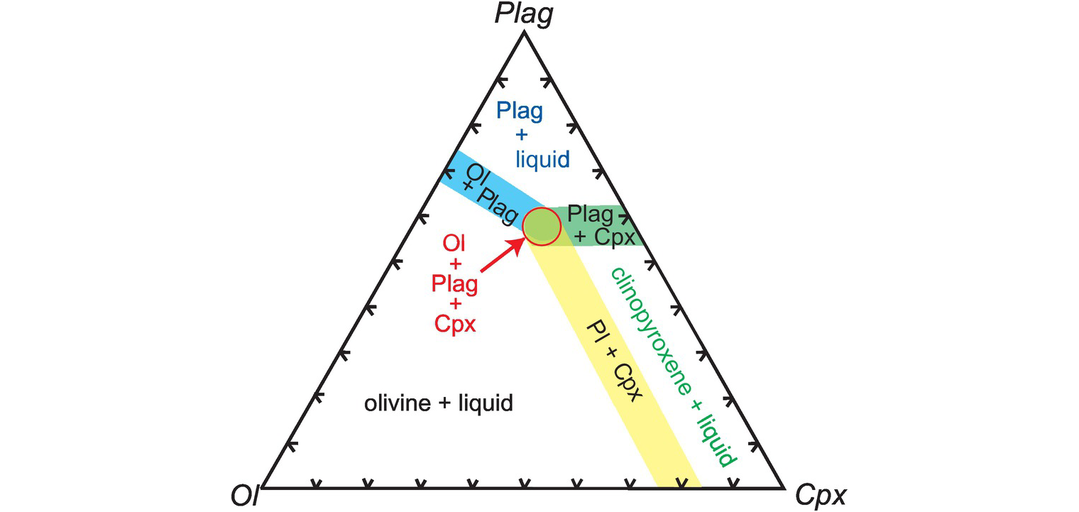
The low-pressure tholeiitic basalt phase diagram of Cox et al. (1979). The projection is from normative quartz onto the critical plane of silica undersaturation in the Yoder–Tilley basalt tetrahedron, modified to olivine–plagioclase–clinopyroxene. Plag = plagioclase, Cpx = clinopyroxene, Ol = olivine.
3.4.1.2 CMAS Diagrams
The components of the CMAS system (CaO–MgO–Al2O3–SiO2) comprise about 70–85 wt.% of most basalts and more than 90 wt.% of most mantle peridotites. Consequently, the CMAS system is used by experimental petrologists as a simplified analogue of more complex basalt and mantle systems. The CMAS projection (Figure 3.26a) provides an excellent framework in which the possible melting behaviour of upper mantle materials may be discussed and is a powerful tool in constructing petrological models. It also may be used to compare the chemistry of particular rock suites with experimentally determined phase boundaries at low and high pressure. Partial melting trends may be identified from a linear array of rock compositions projecting through the plotted source composition and fractional crystallisation trends may be identified as linear arrays projecting through the composition of the fractionating phase(s). The CMAS tetrahedron has apices in a different orientation from those of the tholeiitic component of the Yoder–Tilley tetrahedron. Mineral phases plotted in CMAS space are abbreviated as follows:
All Fe–Ni–Mg olivines as forsterite = M2S
Enstatite; = MS
All feldspar is projected as equivalent anorthite = CAS2
All hercynite, ulvospinel, magnetite and chromite projected as spinel = MA
All garnet plots along the grossular = C3AS3– pyrope M3AS3 join
All clinopyroxenes along the diopside = CMS2–Ca-Tschermak’s molecule = CAS join
(a) Projecting rock compositions into CMAS. The CMAS system (Figure 3.26a) was first used for mantle and basaltic compositions by O’Hara (1968), who proposed a polybaric phase diagram for dry natural basalts and ultramafic rocks up to pressures of 30 kb. He devised a scheme whereby natural rock compositions could be presented in such a way as to be directly comparable with experimental results in the CaO–MgO–Al2O3–SiO2 (CMAS) system. Weight % oxides are converted to molecular proportions and the plotting parameters are calculated as follows:
Cox et al. (1979) gives the equations for CMAS projections as follows:
1. For projection from the olivine projection onto the plane CS–MS–A:
2. For projection from orthopyroxene into M2S–C2S3–A2S3:
3. For projection from diopside into C3A-M-S:
where p is the amount of olivine required to bring the rock into the required plane (this can be a positive or negative amount); c, m, a and s are the calculated values for C, M, A and S for the rock as calculated above; and x, y, z when recast as a percentage are the plotting parameters required for CS, MS and A, respectively.
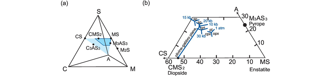
(a) The CMAS tetrahedron for the projection of basaltic and mantle compositions showing the relative positions of the main phases and planes of projection. (b) Projection from olivine (M2S) onto the plane CS–MS–A in the CMAS system showing invariant peritectic points for 1 atm, and 10, 15, 20 and 30 kb. The olivine–gabbro plane divides the diagram into nepheline normative compositions (enstatite-poor) and tholeiitic compositions (enstatite-rich). The stability fields of the different phases are indicated (pl = plagioclase; opx = orthopyroxene; cpx = clinopyroxene; sp = spinel; grt = garnet); in addition, all fields include olivine.
Rock compositions are usually displayed in one of three projections, chosen to include the important mineral phases and to minimise any distortion from the projection. The most used projections are:
(a) from olivine into the plane CS–MS (enstatite) –A
(b) from enstatite into the plane M2S–A2S3–C2S3
(c) from diopside into either the plane C3A–M–S or CA–M–S.
The olivine projection plane contains the pyroxene and garnet solid solutions (Figure 3.26b). The olivine–plagioclase piercing point (not shown) is the point at which the olivine–plagioclase join cuts the CS–MS–A plane, and the line which joins this piercing point to diopside (the olivine–gabbro plane) is the plane of silica saturation (Figure 3.26b). This olivine–gabbro plane divides the diagram into Ne-normative compositions on the enstatite-poor side and tholeiitic compositions on the enstatite-rich side. An example of the calculation procedure for projecting a basaltic composition from olivine onto the CS–MS–A plane is given in Table 3.9. France et al. (2009) have created a software package which converts oxide proportions into CMAS coordinates and allows the visualisation of the results in 3D.
(b) Interpreting CMAS diagrams. For a projection to be useful in interpreting crystal–liquid equilibria it must be made from a phase which is present in the melt; otherwise, the observed trends are meaningless. Second, the projection should not be made from a phase at an oblique angle to the projection plane, otherwise trends which are simply a function of the oblique projection can be misinterpreted and given geological significance where there is none. In addition, although the CMAS projection uses all of the chemical constituents of a rock analysis, the effects of individual components cannot be easily identified. It is important to note that small uncertainties in the chemical analysis may translate into large shifts in the projected compositions. This is particularly acute for uncertainty associated with Na2O and SiO2, where the direction of shift is parallel to an identified fractional crystallisation trend. Thus Presnall et al. (1979) and Presnall and Hoover (1984) make the point that some fractional crystallisation trends observed in ocean-floor tholeiitic glasses could be an artefact resulting from analytical uncertainties magnified by the projection procedure.
(c) An expanded CMAS system. More complex systems which are closer to natural samples include the addition of Na2O and FeO and hence the CMASN and CMASF systems, respectively. Herzberg and O’Hara (2002) describe a more complete, expanded version of the CMAS plot which incorporates other elements and brings the projection more into line with the Yoder and Tilley type plots described above. They show that the addition of the components TiO2, Cr2O3, FeO, MnO, Na2O, K2O and NiO can expand and contract liquidus crystallisation fields, although the replacement of MgO by FeO does not change crystallisation fields greatly.
| Wt.% oxide of rock | Molecular weight | Molecular proportions | ||||
|---|---|---|---|---|---|---|
| SiO2 | 46.95 | 60.09 | 0.7813 | |||
| TiO2 | 2.02 | 79.9 | 0.0253 | |||
| Al2O3 | 13.1 | 101.96 | 0.1285 | |||
| Fe2O3 | 1.02 | 159.69 | 0.0064 | |||
| FeO | 10.07 | 71.85 | 0.1402 | |||
| MnO | 0.15 | 70.94 | 0.0021 | |||
| MgO | 14.55 | 40.3 | 0.3610 | |||
| CaO | 10.16 | 56.08 | 0.1812 | |||
| Na2O | 1.73 | 61.98 | 0.0279 | |||
| K2O | 0.08 | 94.2 | 0.0008 | |||
| P2O5 | 0.21 | 141.95 | 0.0015 | |||
| TOTAL | 100 | |||||
| CMAS plotting parameters | ||||||
| C = | 13.110 | |||||
| M = | 19.265 | |||||
| A = | 43.493 | |||||
| S= | 43.493 | |||||
| Projection parameters for olivine projection into CS–MS–A using the equation of Cox et al. (1979) | ||||||
| Balance the equation rock + p.olivine = x.CS + y.MS + z.A | ||||||
| CcMmAaSs + p.M57.3S42.7 = x.C48.3S51.7 + y.M40.1S59.9 + z.A100 | ||||||
| Balancing C | 48.3x = 13.11 | |||||
| Balancing M | 40.1y = 50.73p + 19.269 | |||||
| Balancing A | 100z = 19.261 | |||||
| Balancing S | 51.7x + 59.9y = 43.493 + 42.7p | |||||
| % | ||||||
| CS | x = | 0.271 | 27.95 | |||
| MS | y = | 0.507 | 52.21 | |||
| A | z = | 0.193 | 19.84 | |||
| sum = | 0.971 | |||||
In this expanded version of CMAS the diopside projection onto the plane olivine–anorthite–quartz requires all wt.% compositions be converted to mole % and any Fe2O3 combined with diopside so that the precise point of projection is diopside + Fe2O3 + Na2O.Si3O6 + K2O.Si3O6. The projection coordinates are calculated in the following way (Herzberg and O’Hara, 2002):
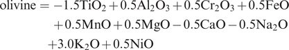
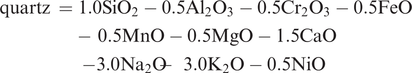
An example of the projection is given in Figure 3.27 (after Herzberg et al., 2007).
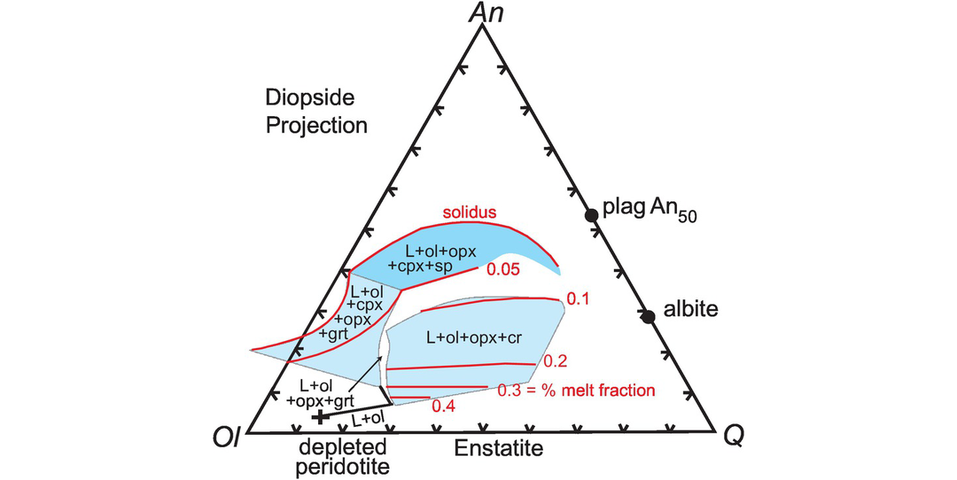
The diopside projection of the expanded CMAS system showing the projection of liquid compositions (mole percent) in equilibrium with depleted mantle peridotite from diopside + Fe2O3 + Na2O.Si3O6 + K2O.Si3O6 onto the plane olivine–anorthite–silica. Red lines show the contours of equal melt fractions (after Herzberg et al., 2007; with permission from John Wiley & Sons). L = liquid, ol = olivine, cpx = clinopyroxene, sp = spinel, grt = garnet, cr = chromite, plag = plagioclase.
3.4.1.3 FeO–MgO Plots
Many mafic and ultramafic rocks have experienced olivine fractionation – both the removal or accumulation of olivine – and thus it can be difficult to establish the composition of the initial primary magma. In order to solve this problem Herzberg and O’Hara (2002) parameterised a large experimental database for mantle peridotites to explore the effects of equilibrium melting, fractional melting and peridotite source composition on the FeO and MgO content of potential primary mantle melts. This work has particular relevance to the study of magnesian basalts, MORB, picrites and komatiites and, when coupled with further experimental data, has the potential to provide information on the depth of melting and the mantle potential temperature of primary mantle melts (see Herzberg et al., 2007).
Herzberg and O’Hara (2002) showed that MgO and FeO in a mantle melt are both highly sensitive to differing source compositions, pressure of melting and degree of melting. For a range of different mantle compositions which include fertile and depleted mantle peridotite and Fe-rich and Fe-poor peridotite they calculated melt compositions which are in equilibrium with a harzburgitic residue (olivine + orthopyroxene) and with olivine, and show how they vary in MgO–FeO space with variations in the mode of melting (equilibrium melting and accumulated fractional melting), the degree of melting (the melt fraction) and the depth of equilibration (pressure in GPa). An example of their approach is shown in Figure 3.28a which is based on a fertile, low-Fe peridotite (KR-4003, Kettle River peridotite) with a composition very similar to that of the primitive mantle of McDonough (2014a) described in Table 3.2. In detail the approach employs the extrapolation of the results of melting experiments on a given peridotite composition using existing exchange coefficient data for olivine and orthopyroxene in mafic and ultramafic melts together with mass balance considerations.
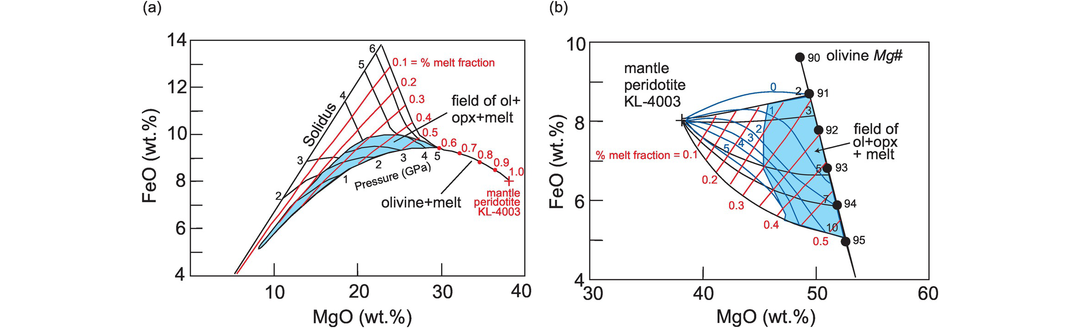
FeO–MgO plots for mantle melting showing how melt compositions vary according to the melt fraction, the pressure of initial melting and the final pressure of melting. (a) Partial melt compositions from the accumulated fractional melting of mantle peridotite KL-4003, a peridotite similar in composition to the primitive mantle. The shaded area shows the field of melts in equilibrium with a harzburgite residue (ol + opx + melt) and to the right are melts in equilibrium with olivine. Red lines show partial melt fractions and the black lines show the pressure of initial melting in GPa (after Herzberg and O’Hara, 2002; by permission of Oxford University Press). (b) The composition of model melt residues formed after the fractional melting of peridotite KL-4003. The olivine line shows the field for dunite residues, the shaded area shows the field of harzburgite residues (ol + opx + melt) and the area to the left is the field of spinel/garnet peridotite residues. The heavy black line shows the composition of olivine in dunite residues with the olivine Mg# values indicated. The black lines show the initial pressure of melting, the blue lines show the final pressure of melting, and the red lines show percent melt fraction (after Herzberg, 2004; by permission of Oxford University Press). ol = olivine, opx = orthopyroxene.
In order to apply this parameterisation to a cogenetic suite of magnesian melts in equilibrium with olivine, Herzberg and O’Hara (2002) provide an ‘inverse model’. This method consists of selecting a representative lava composition in which olivine has a composition in equilibrium with the melt. Olivine is then incrementally added or subtracted in 1 wt.% increments from the melt (see Herzberg and O’Hara, 2002, appendix 5). The suite of calculated compositions is transferred onto the FeO–MgO plot and compared with the range of liquid compositions computed (see Herzberg et al., 2007, appendix A). A unique solution is found when the liquid along the olivine addition–subtraction line displays a common melt fraction in FeO–MgO space and in either another two-dimensional plot such as MgO–SiO2 or a projection in CMAS space (Figure 3.26). It is important to note that this method is sensitive to the accurate estimation of the Fe3+/Fe2+ ratio of the melt.
Residual peridotite compositions are also a function of initial and final decompression pressures and Herzberg (2004) computed the fields of residual peridotites formed in equilibrium with basaltic melts using the experimental data of Walter (1998) for fertile peridotite KR-4003 and mass balance calculations. Model residue compositions from fractional melting are shown in Figure 3.28b for dunites (see the range of olivine compositions) and harzburgites (the field of olivine + orthopyroxene) and garnet and spinel lherzolites for initial melting pressures between 2 and 10 GPa and final melting pressures of between 0 and 5 GPa for a range of melt fractions.
3.4.2 Melting Mafic Crust
Experimental studies show that when mafic rocks melt, the composition of the melt tends to be felsic and this is particularly relevant when the melting takes place in the presence of water. However, since most mafic rocks are very low in potassium, the derived felsic melts tend to be more sodic than typical granites and fall in the compositional range of tonalites, trondhjemites and granodiorites. It is this observation which has led many geochemists to infer that the Earth’s early continental crust which is predominantly tonalite–trondhjemite–granodiorite (TTG) in composition was primarily formed through the melting of mafic crust, either at the base of a thickened crust or in a subduction setting (Rollinson, 2007). Studies of oceanic plagiogranites also suggest that some may be the product of partial melting of mafic oceanic crust (see Rollinson, 2009).
The most common way to express the melting of mafic rocks is on the ‘granite’ normative An–Ab–Or diagram described in Section 3.2.2. Rock compositions are most often recalculated using the CIPW norm and the An–Ab–Or components recast as 100%, then plotted on the ternary diagram as outlined in Section 3.2.2. This is illustrated in Figure 3.29 which shows the locus of calculated compositions from the water-saturated melting of an enriched Archaean tholeiite. These compositions were calculated from the results of thermodynamic equilibrium modelling in the ten-component NCKFMASHTO system using the THERMOCALC software of Powell and Holland (1988). In detail the results of experimental studies vary quite widely, not just as a result of pressure and temperature of melting, but also as a consequence of the extent to which water is included in the melting process and the chemical composition of the basaltic starting material. A more extensive range of felsic melt compositions produced in basalt melting experiments is given in Johannes and Holz (1996).
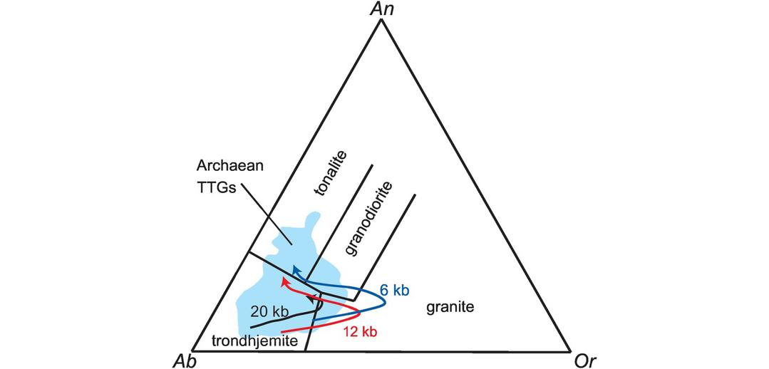
The normative An–Ab–Or plot with compositional fields of Barker (1979). Calculated compositions from water-saturated melting of an enriched Archaean tholeiite with increasing temperature (arrow) from the solidus at 600–700°C to 1000°C (head of arrow) for three different pressures (6, 12 and 20 kb). The results are compared with the compositional field of an Archaean tonalite–trondhjemite–granodiorite (TTG) suite.
3.4.3 Melting Felsic (Continental) Crust
Classical studies in the 1950s sought to understand the origin of granitic crust in terms of the melting behaviour of potassic granites. Experiments were constructed to understand the behaviour of granites and rhyolites during their initial melting or final stages of crystallisation in which the major part of the rock compositions could be reduced to the normative minerals quartz, albite and orthoclase. In recent decades the approach has become different, for we now assume that felsic rocks in general, and granites and rhyolites in particular, are for the most part the product of partial melting of pre-existing sialic crust such as metamorphosed sediments or pre-existing granites or ‘granitic’ gneisses. In addition, some felsic rocks are the product of the partial melting of mafic rocks, as discussed in Section 3.4.2, and in rare cases the product of crystal fractionation of mafic rocks. This has led to some new questions about the genesis of granitic rocks. First is the question of the protolith: What melted? Second, what were the melting reactions which controlled the composition of the melts that were produced (e.g., Weinberg and Hasalova, 2015)? Pertinent to this discussion is the extent to which water and other volatiles facilitated or inhibited the partial melting process. Was the melting process ‘dry’ or was it facilitated by the presence of water, supplied either from the breakdown of hydrous phases such as the micas and amphiboles in the protolith or from an external supply? Finally, to what extent is a given felsic rock composition representative of a melt? In the case of glassy rocks or melt inclusions the answer is straightforward, but it is possible that many granitic rocks contain restitic materials from their source which did not melt. Some granites therefore may contain ‘parental’ phenocrysts, or xenocrysts, which will distort the rock composition from that of a primary melt.
3.4.3.1 The Normative Albite–Orthoclase–Quartz Diagram: The ‘Granite System’
In 1958 Tuttle and Bowen demonstrated a marked coincidence between the compositions of natural rhyolites and granites containing more than 80 wt.% normative albite, orthoclase and quartz and the normative compositions of experimentally determined minima and eutectics in the system albite–orthoclase–quartz–H2O. This system is sometimes known as the haplogranite system. Their observations provided a way for igneous petrologists to attempt to correlate experimental information with analytical data projected into the system Ab–Or–Q–H2O. Tuttle and Bowen (1958) and subsequent workers determined the compositions at which the phases quartz, orthoclase and albite coexist with a water-saturated melt at a variety of pressures (Table 3.10) and plotted their results as a projection onto the anhydrous base of the Ab–Or–Q–H2O tetrahedron. The plotting procedure requires three steps:
2. Summation of the normative values of albite, orthoclase and quartz
3. Recasting of these values as a percentage of their sum.
These values are plotted on a ternary diagram. The results of these experiments show that the quartz–alkali feldspar boundary moves away from the quartz apex with increasing pressure from 1 to 10 kb (Figure 3.30a). Accompanying this expansion is the increased solubility of water in the melt (see Table 3.10). A lesser expansion is observed between 10 and 30 kb (Figure 3.23b). At approximately 3.5 kb and 660°C the quartz–alkali feldspar field boundary intersects the crest of the alkali feldspar solvus and the liquid at this point coexists with quartz, orthoclase and albite (Merrill et al., 1970). At 30 kb the assemblage is coesite, sanidine hydrate and jadeiite. Thus, a direct comparison can be made between experimentally determined phase boundaries and natural rock compositions. A synthesis of much of the relevant experimental work is given in the text by Johannes and Holz (1996) and a summary of the locus of the minima and eutectics for the water saturated system is given in Figure 3.30b.
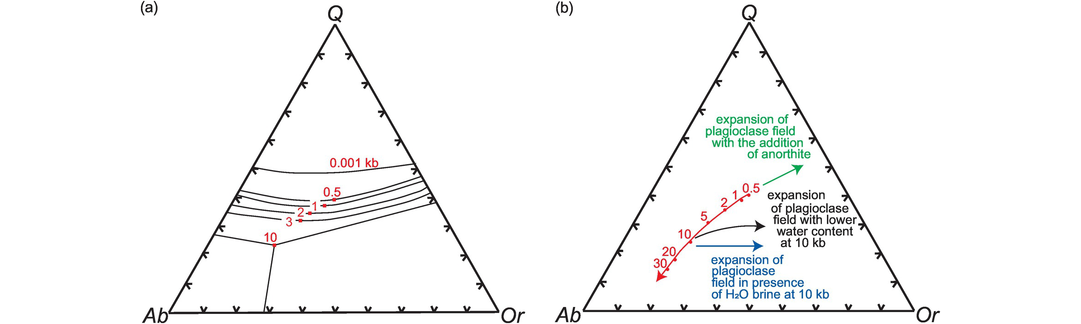
The haplogranite system. (a) Cotectics, minima and eutectics (red squares) for the water-saturated haplogranite system (Q–Ab–Or–H2O, wt.%) at a range of pressures (after Blundy and Cashman, 2001; adapted by permission from Springer-Nature). (b) Minima and eutectics in the Q–Ab–Or–H2O system projected from H2O onto the plane Ab–Q–Or for 0.5–30 kb pressure (red circles). Also shown are the trajectories for undersaturated melts at 10 kb (black arrow), melts in equilibrium with H2O-brines (blue arrow) and the expansion of plagioclase phase volume with the addition of anorthite to the system (green arrow), after Aranovich et al. (2013). Data for water-saturated system at 1 kb from James and Hamilton (1969).
| Pressure (kb) | Temperature (°C) | Composition (wt.%) | H2O (wt.%) | X H2O | Reference | ||||||
|---|---|---|---|---|---|---|---|---|---|---|---|
| Ab | Or | Q | |||||||||
| SYSTEM: ALBITE–ORTHOCLASE–QUARTZ–H2O | |||||||||||
| 0.001 | 990 | 33 | 33 | 34 | 0.0 | 1.00 | Minimum | Schairer and Bowen (1935) | |||
| 0.500 | 770 | 30 | 30 | 40 | 3.0 | 1.00 | Minimum | Tuttle and Bowen (1958) | |||
| 1.000 | 720 | 33 | 29 | 38 | 4.4 | 1.00 | Minimum | Tuttle and Bowen (1958) | |||
| 2.000 | 685 | 39 | 26 | 35 | 6.5 | 1.00 | Minimum | Tuttle and Bowen (1958) | |||
| 2.000 | 685 | 39 | 25 | 36 | 6.5 | 1.00 | Minimum | Holz et al. (1992) | |||
| 2.000 | 775 | 36 | 29 | 35 | 3.6 | 0.70 | Minimum | Holz et al. (1992) | |||
| 2.000 | 830 | 34 | 31 | 35 | 2.5 | 0.50 | Minimum | Holz et al. (1992) | |||
| 3.000 | 665 | 42 | 25 | 33 | 8.3 | 1.00 | Minimum | Tuttle and Bowen (1958) | |||
| 4.000 | 1000 | 32 | 34 | 34 | 0.0 | 0.00 | Minimum | Steiner et al. (1975) | |||
| 3.923 | 665 | 9.7 | 1.00 | Eutectic | Tuttle and Bowen (1958) | ||||||
| 4.000 | 655 | 47 | 23 | 30 | 9.9 | 1.00 | Eutectic | Steiner et al. (1975) | |||
| 5.000 | 640 | 50 | 23 | 27 | 11.0 | 1.00 | Eutectic | Luth et al. (1964) | |||
| 5.000 | 645 | 47 | 22 | 31 | 11.0 | 1.00 | Eutectic | Holz et al. (1992) | |||
| 5.000 | 735 | 43 | 25 | 32 | 4.0 | 0.85 | Minimum | Holz et al. (1992) | |||
| 5.000 | 790 | 40 | 28 | 32 | 3.0 | 0.70 | Minimum | Holz et al. (1992) | |||
| 5.000 | 756 | 43 | 30 | 27 | 4.1 | 0.50 | Minimum | Ebadi and Johannes (1991) | |||
| 5.000 | 990 | 35 | 33 | 32 | 1.0 | 0.07 | Minimum | Becker et al. (1998) | |||
| 8.000 | 1050 | 37 | 34 | 29 | 1.0 | ~0.1 | Minimum | Holz et al. (1992) | |||
| 10.000 | 620 | 56 | 21 | 23 | 17.0 | 1.00 | Eutectic | Luth et al. (1964) | |||
| 10.000 | 1070 | 26 | 45 | 29 | 0.0 | 0.00 | Minimum | Huang and Wyllie (1975) | |||
| 20.000 | 630 | 63 | 19 | 18 | 21.0 | 1.00 | Eutectic | Huang and Wyllie (1975) | |||
| 30.000 | 680 | 67 | 18 | 15 | 24.5 | 1.00 | Eutectic | Huang and Wyllie (1975) | |||
| SYSTEM: ALBITE–ORTHOCLASE–QUARTZ–ANORTHITE–H2O | |||||||||||
| 1 | 730 | 32 | 29 | 39 | An3 plane | nd | Piercing point | James and Hamilton (1969) | |||
| 1 | 745 | 22 | 36 | 42 | An5 plane | nd | Piercing point | James and Hamilton (1969) | |||
| 1 | 780 | 11 | 42 | 47 | An7.5 plane | nd | Piercing point | James and Hamilton (1969) | |||
| SYSTEM: ALBITE–ORTHOCLASE–QUARTZ–H2O–F | |||||||||||
| 1 | 690 | 45 | 26 | 29 | 1% F | ca 4.0 | Minimum | Manning (1981) | |||
| 1 | 670 | 50 | 25 | 25 | 2% F | ca 4.0 | Minimum | Manning (1981) | |||
| 1 | 630 | 58 | 27 | 15 | 4% F | ca 4.0 | Eutectic | Manning (1981) | |||
Note: nd = not determined.
Many experimental studies following the early work of Tuttle and Bowen (1958) focussed on the effect of water on melting conditions in the haplogranite system – in particular, melting under water-undersaturated conditions. The results summarised in Table 3.10 and Figure 3.30 show two main effects: (i) the position of the cotectic curve does not alter significantly, but the temperature of melting increases as melting approaches dry conditions and (ii) the minimum shifts towards the quartz–orthoclase boundary and the relative volume of albite expands at the expense of orthoclase as the volume of quartz remains constant (Figure 3.30b). More recent studies show a similar, although more extreme shift, accompanying the presence of NaCl–KCl brines during melting (Aranovich et al., 2013).
The addition of anorthite to the ‘granite’ system expands the phase volume of plagioclase and shifts compositions into the granodiorite and tonalite fields. This was investigated by James and Hamilton (1969) at 1 kb, who found that the position of the piercing point minimum shifts towards the quartz–orthoclase boundary of the projection with increasing anorthite, indicating an increase in the primary phase volume of plagioclase (Figure 3.30b).
Petrologists have used the haplogranite system to explore the processes of crustal differentiation during anataxis and the genesis of plutonic felsic rocks, as well as the ascent and crystallisation of felsic volcanic rocks. For example, Blundy and Cashman (2001) used glass compositions preserved in dacitic magmas from Mount St Helens to distinguish between ascent-driven and cooling-driven crystallisation. Their work supports a view of polybaric fractional crystallisation, indicating that there are limits to the use of isobaric experiments on their own. Cesare et al. (2015) and Acosta-Vigil et al. (2017) used melt inclusion data, combined with experimental diffusion studies of granitic melts plotted relative to experimentally determined phase boundaries in the haplogranite system, in order to explain the processes of partial melting in the middle and lower continental crust.
3.4.3.2 Partial Melting of Crustal Rocks
Experimental studies of crustal melting focus on the melting of meta-sediments (pelites and meta-greywackes) and pre-existing volcanic and plutonic felsic rocks and their gneissose equivalents. The results of these studies are typically plotted on the normative wt.% ‘granite’ An–Ab–Or diagram (Section 3.2). Typically, crustal melting is facilitated by the presence of water derived during the dehydration of the protolith (dehydration melting) or from water fluxing (fluid-present or water-present melting). Weinberg and Hasalova (2015) provide a helpful review of the physical and petrological processes which are involved and summarise a series of relevant experimental studies with melt compositions plotted on the normative An–Ab–Or diagram. They show that during water-undersaturated melting conditions (dehydration melting) melt compositions are more potassic and plot in the granite and granodiorite fields, whereas water-saturated melting produces more sodic compositions which plot in the trondhjemite field (see Figure 3.31 for a compilation of similar results).
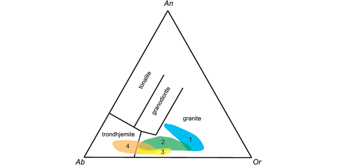
Normative anorthite–albite–orthoclase (wt.%) granite classification diagram of Barker (1979) showing melt fields for felsic igneous rocks and metasediments. 1: Dehydration melting of biotite gneiss (at 3–15 kb, 875–1000°C) (Patino Douce and Beard, 1995); 2: vapour-absent melting of tonalite at ultra-high pressures (at 15–32 kb, 900–1150°C) (Patino Douce, 2005); 3: dehydration melting of muscovite schist and muscovite biotite schist (at 6–10 kb, 750–900°C) (Patino Douce and Harris, 1998); 4: water-fluxed melting of muscovite schist (at 6–10 kb, 700–750°C)
3.4.4 What Melted?
Establishing the nature of the protolith of granite requires a full range of geochemical analyses including major and trace elements, radiogenic isotopes and sometimes stable isotopes. For this reason, major element data on their own can yield only a preliminary indication of the nature of a granitic source – nonetheless, these data can be useful. The two approaches outlined here include the aluminium-saturation index (Frost and Frost, 2008) and the Al–Fe–Mg–Ti–Ca diagrams of Patino Douce (1999).
3.4.4.1 The Aluminium Saturation Index (ASI)
The aluminium saturation index is defined in Section 3.2.4. As summarized there, peraluminous rocks contain more Al than is necessary to make feldspars and this excess Al may show itself as normative corundum (Zen, 1988), as phases in granites such as muscovite and biotite, or if the rock is strongly peraluminous, as one of the aluminosilicates, garnet or cordierite. Rocks with excess Al imply a clay-rich protolith and so might have had a metasedimentary source. Metaluminous rocks with ASI < 1.0, but molecular Na + K < molecular Al, are likely to have an excess of Ca and so may contain calcic phases such as hornblende or clinopyroxene. It is sometimes helpful to make a bivariate plot showing changing ASI versus SiO2 (as illustrated in Figure 3.9).
3.4.4.2 Al–Fe–Mg–Ti–Ca Diagrams
Experimental studies by Patino Douce (1999) show that there are compositional differences between melts of pelites, greywackes and amphibolite in Al–Fe–Mg–Ti–Ca–oxide space. This work is the result of a series of dehydration melting experiments on fertile source rocks containing either biotite and or muscovite in the case of pelites and psammites, and hornblende in the case of amphibolites. Patino Douce’s (1999) fields for partial melts of felsic pelites, psammites and amphibolites show how pelite-derived melts are more aluminous than psammite-derived melts, which in turn are more aluminous than melts from amphibolite (Figure 3.32a). Amphibolite-derived melts are also enriched in FeO, MgO and CaO, relative to pelitic and psammitic melts (Figure 3.32b).
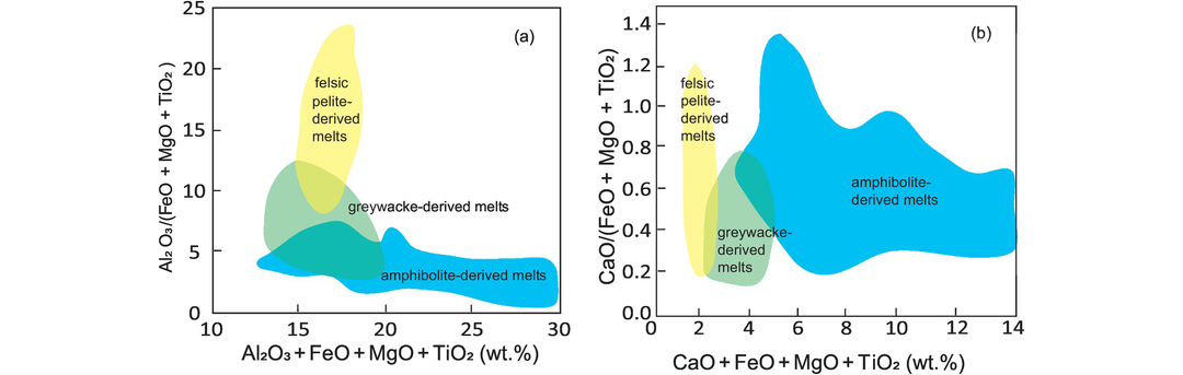
(a) Al2O3/(FeO + MgO + TiO2) versus (Al2O3 + FeO + MgO + TiO2) and (b) CaO/(FeO + MgO + TiO2) versus (CaO + FeO + MgO + TiO2) plots showing the fields of partial melts derived from felsic pelites, greywackes and amphibolites. All oxide values are wt.%.