4.1 Introduction
A trace element may be defined as an element which is present in a rock in concentrations of less than 0.1 wt.%, that is, less than 1000 parts per million (ppm). This means that it is not normally a stoichiometric constituent of the minerals which make up the rock; rather, it substitutes for one of the major elements in the structure of a host mineral. As a consequence of their low abundances, trace elements do not influence the chemical or physical properties of the system. There are, however, some limitations to this definition, for in igneous rocks the elements K and P behave as trace elements in mid-ocean ridge basalts, whereas in granites they form discrete minerals such as K-feldspar and, in the case of P, apatite or monazite. Unlike the major elements whose concentrations in the Earth’s crust vary over a relatively narrow range, the range of trace element concentrations may be several orders of magnitude.
As analytical methods have improved in both the range of elements that can be analysed and in the precision that their concentrations can be measured, trace element studies have become a vital part of modern petrology. This is because of the following:
1. Trace elements are more sensitive to geochemical processes than major elements and are therefore better at discriminating between petrological processes.
2. Their great chemical diversity coupled with the fact that different elements behave in different ways permits a wide range of possible processes to be assessed.
Thus, one of their principal uses is in the identification of geochemical processes. Particularly important is the fact that there are mathematical models to describe trace element distributions which allow the quantitative testing of petrological hypotheses. These are most applicable to processes in magmatic systems which are controlled by crystal–melt or crystal–fluid equilibria, but are also relevant to the processes involved in the formation of meteorites, sediments and ore deposits.
In this chapter we first develop some of the theory behind the distribution of trace elements and explain the physical laws used in trace element modelling. Then various methods of displaying trace element data are examined as a prelude to showing how trace elements might be used in identifying geological processes and in testing hypotheses.
4.1.1 The Classification of Trace Elements According to Their Geochemical Behaviour
A frequently used classification of the elements based upon their geochemical behaviour was proposed by Goldschmidt (1937), often regarded as the ‘father of geochemistry’. He proposed a fourfold classification, the nomenclature for which is still largely in current use:
To this quartet has been added (Lee, 2016):
Apart from the term ‘atmophile’, which is almost never used, this nomenclature is still in use today albeit with slightly different meanings. It is important to note, however, that some elements will demonstrate more than one type of geochemical behaviour.
A further classification of elements which is widely discussed is the cosmochemical classification relating to processes of planetary accretion. In this case elements are classified according to their condensation temperature from gaseous to solid or liquid state during the cooling of a solar nebula. This classification is relevant to the formation of meteorites and the earliest stages of Earth formation, and so is useful when discussing large-scale planetary features, although is less relevant when considering crust and mantle geochemistry. Elements are grouped as follows according to condensation temperature in kelvin (K):
Highly refractory (>1700 K), to include Re, Os, W, Zr and Hf
Moderately refractory (1300–1500 K), to include Mg, Si, Cr, Fe, Co and Ni
Moderately volatile (1100–1500 K), to include Cu, Ba and Mn
Volatile (700–1100 K), to include Na, K, S and Rb
Highly volatile (<700 K), to include Pb, O, C, N, H and noble gases
Trace elements are often studied in groups, and deviations from group behaviour or systematic changes in behaviour within the group are used as an indicator of petrological processes. The association of like trace elements also helps to simplify what can otherwise be a very unwieldy data set. Most geochemically important trace elements can be classified either on the basis of their position in the periodic table or according to their behaviour in magmatic systems, as discussed below.
4.1.1.1 Trace Element Groupings in the Periodic Table
Goldschmidt‘s geochemical classification of the elements presented above can be interpreted in terms of location within the periodic table. Here specific elemental groups are highlighted for their particular importance in trace element geochemistry (Figure 4.1). The most obvious in this respect are the lanthanides, elements with atomic numbers 57–71 (La to Lu), or the rare earth elements (REE) as they are usually called in geochemistry. Y also behaves in a manner similar to the REE. The platinum group elements (PGE, or platinum group metals, PGM) include elements with atomic numbers 44–46 – Ru, Rh, Pd – and 76–79 – Os, Ir, Pt. They are known as the noble metals if they also include Au. An expanded grouping of the PGE is known as the highly siderophile elements (HSE) and includes Os, Ir, Ru, Rh, Pt and Pd, together with Re and Au, which have some similar properties. This group can be used in understanding the large-scale processes associated with planetary accretion and differentiation, in particular, core formation, due to their affinity for metal relative to silicate minerals. The term transition metals (atomic numbers 21–30, Sc–Zn) is usually restricted to the first transition series and includes the two major elements Fe and Mn.
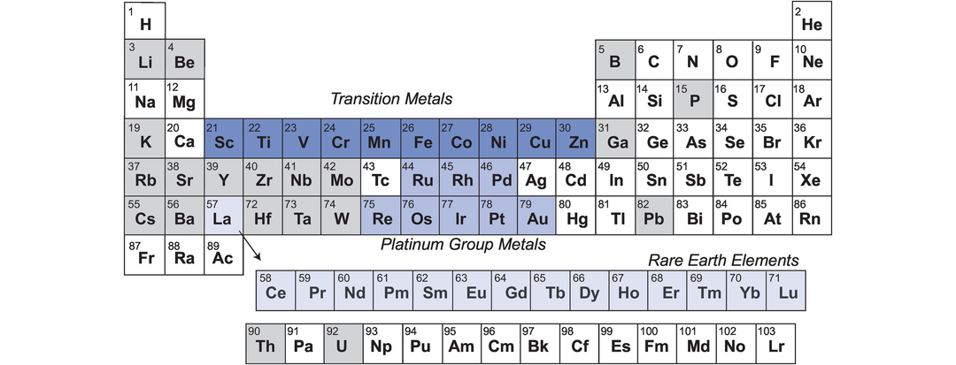
The periodic table of the elements. The three main groups of trace elements which are treated together in geochemistry because of their relative positions on the periodic table are highlighted. These are the elements of the first transition series (transition metals), the platinum group elements + Re and Au (platinum group metals) and the rare earth elements. Other trace elements important in geochemistry are shaded light grey.
The elements in each of these respective groups have similar chemical properties and for this reason are expected to show similar geochemical behaviour. However, this may not always be the case, for geological processes can take advantage of subtle chemical differences within an elemental group and fractionate elements one from the other. Thus, one of the tasks of trace element geochemistry is to discover which geological processes may have this effect and to quantify the extent of particular processes.
4.1.1.2 Trace Element Behaviour in Magmatic Systems
When the Earth’s mantle is melted, trace elements display a preference either for the melt phase or the solid (mineral) phase. Trace elements whose preference is the mineral phase are described as compatible, whereas elements whose preference is to remain in the melt are described as incompatible; in other words, they are incompatible in the mineral structure and will leave at the first available opportunity. In detail there are degrees of compatibility and incompatibility, and so trace elements may be described as moderately incompatible or highly incompatible. The degree of trace element incompatibility is quantified by the mineral-melt partition coefficient (see Section 4.2.1). Trace element incompatibility is also the basis for the ordering of elements in mantle normalised trace element diagrams (see Section 4.4). The degree of incompatibility will vary between melts of different compositions. For example, P is incompatible in mantle minerals and during partial melting will be concentrated in the melt. In granites, however, even though P is present as a trace element it is compatible because it is accommodated in the structure of the accessory mineral phases apatite and monazite.
It is sometimes helpful to subdivide the incompatible elements on the basis of their charge to size ratio. This property is often described as the field strength and may be thought of as the electrostatic charge per unit surface area of the cation. It is also described as the ionic potential of an element and is quantified as the ratio of the valence to the ionic radius, which is measured in picometres. Figure 4.2 shows a plot of ionic size versus charge for a range of trace elements. In addition, some major elements are shown to indicate where atomic substitutions most commonly occur. Small highly charged cations located in the lower right of the diagram are known as high field strength (HFS) cations (ionic potential > 0.02). The broadest definition of HFS elements (HFSE) includes the trivalent REE, Y, Sc, Th, U and the PGE, although more commonly the term is restricted to those elements that are tetravalent (Hf, Ti, Zr), pentavalent (Nb, Ta) and hexavalent (W, Mo). With the exception of Mo, the HFS elements are commonly fluid immobile and therefore their concentrations normally remain unchanged during weathering or metamorphism.
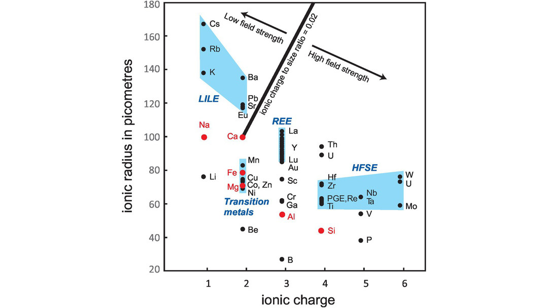
Plot of ionic radiius (measured in picometres, 10−12 m) versus ionic charge for incompatible trace elements of geological interest. Major elements (in red) indicate where trace element ionic substitutions will most readily occur. An ionic potential (charge to size ratio) of 0.02 subdivides the incompatible elements into low field strength (LFS) elements (also known as large ion lithophile elements, LILE) and high field strength elements (HFSE). The ionic radii are from Shannon (1976) and are quoted for six-fold coordination to allow a comparison between all elements.
Elements with ionic radii too large to fit into most silicate minerals and with a small charge are known as low field strength cations (ionic potential < 0.02). They are also known as the large ion lithophile elements (LILE) and are primarily the alkali and alkali earth elements (Figure 4.2). The term ‘LILE’ has been used in a number of different ways, but Chauvel and Rudnick (2018) recommend that the term be restricted to lithophile trace elements having large radius to charge ratios and which have ionic radii greater than those of Ca2+ and Na1+ (100 and 102 picometers, respectively) – these are the largest cations commonly found in rock-forming minerals. By this definition, the list of LILE is restricted to K, Rb, Sr, Cs, Ba, Pb2+ and Eu2+. LILE elements are commonly fluid mobile elements, and so their primary concentrations may change during post-solidus alteration.
Other important trace elements include the following:
The small cations such as Li+, Be2+, B3+, P5+ which are all moderately incompatible.
Ga, which substitutes for Al and so is concentrated in Al-rich minerals in the crust; during partial melting of the mantle, Ga is incompatible in most phases, including garnet, but is compatible in spinel (Davis et al., 2013).
Although not trace elements, volatiles with low solubility such as CO2 in mafic melts may also behave as trace elements (Saal et al., 2002).
Some elements have very similar charge and size, and observing their geochemical behaviour can be particularly important. These include the following elements:
Hf and Zr, and Nb and Ta; both element pairs are almost identical in size and charge and show very similar geochemical behaviour. Nevertheless, in some circumstances the element pairs are fractionated; thus, the ratios Hf/Zr and Nb/Ta are important geochemical parameters.
U and Th have a similar charge and size and both are highly incompatible in magmatic systems but may be fractionated with Th being the more incompatible; U/Th may also be fractionated during fluid–rock interaction.
Amongst the low field strength, large ion lithophile cations, Sr, divalent Eu and divalent Pb have almost identical ionic radii and charge.
A version of the ionic charge to size ratio diagram is given by Chauvel (2018) contoured for element incompatibility in the mineral clinopyroxene. The diagram shows that the most compatible elements are those with an ionic charge and size closest to the major cations in the host mineral (in this case, divalent Ca, Mg and Fe). Incompatibility increases with the difference in charge and size from that of the major cations, such that the monovalent LILE and the pentavalent HFSE are highly incompatible.
4.1.1.3 Trace Elements of Economic Significance
Some trace elements may have strategic importance in local economies and these have become known as the critical metals. These are metals that are economically important for industry but their supply may be limited because they can be obtained from only a few locations worldwide (Moss et al., 2011). They include elements such as the REE, the PGE, Ga, Sb, In, Be, Co, W, Nb and Ta. The critical metals are important in the electronics industry, and a subset of them, known as the E-tech elements, are important in the development of renewable energy technologies (Grandell et al., 2016). These elements include Co, Ga, In, Te, Li and the heavy REE (HREE). Some of these elements, such as indium (In, atomic number 49) and tellurium (Te, atomic number 52), are very rare and not well understood geochemically.
4.2 Physical Controls on Trace Element Distribution
Modern quantitative trace element geochemistry assumes that trace elements are present in a mineral in solid solution through substitution. The principal variables are the charge and size of the trace ion relative to the charge and size of the lattice site. These properties were recognised by Goldschmidt (1937), who through empirical observation proposed a series of qualitative rules to govern the priority which is given to ions with similar charge and size competing to enter a given crystal lattice. However, modern studies of trace element partitioning have shown that Goldschmidt’s rules are not universally correct, for it is also necessary to also consider the energetics of the crystal lattice itself (Blundy and Wood, 2003; also see Section 4.2.1.2).
More recently, this approach has been quantified and trace element distributions are now described in terms of equilibrium thermodynamics. Trace elements may mix in their host mineral in either an ideal or a non-ideal way. Their very low concentrations, however, lead to relatively simple relationships between composition and activity. When mixing is ideal, the relationship between activity and composition is given by Raoult’s law, that is,
where ai is the activity of trace element i in the host mineral and Xi is its composition.
If the trace element interacts with the major components of the host mineral, the activity will depart from the ideal mixing relationship, and at low concentrations the activity composition relations obey Henry’s law. This states that at equilibrium the activity of a trace element i in mineral j (aij) is directly proportional to its composition:
where kij is the Henry’s law constant – a proportionality constant (or activity coefficient) for trace element i in mineral j and where Xij is small. In fact, White (2013) suggests that adherence to Henry’s law can be a helpful way of defining a trace element.
A detailed study by Drake and Holloway (1981) demonstrated that for elements that are homovalent (of identical charge) Henry’s law seems to apply through a wide range of trace element concentrations. Similarly, Wood and Blundy (1997) showed that REE partitioning in clinopyroxene follows Henry’s law behaviour even though the REE concentrations in clinopyroxene ranged from tens to thousands of ppm. However, where the substitutions are heterovalent and the mineral structure has to be electrostatically balanced either through a vacancy or an ion with a balancing charge, then Henry’s law may not always apply. In this case, partitioning may depend upon the concentration of specific ions. For example, Grant and Wood (2010) showed this to be the case for Sc partitioning in olivine in which DolSc (the partition coefficient for Sc between olivine and melt) varied according to the concentration of Sc in the melt. Henry’s law also ceases to apply at very high concentrations, although the point at which this takes place cannot be easily predicted and must be determined for each individual system. For example, Prowatke and Klemme (2006) demonstrated that Sm partitioning into titanite showed a dependence on the bulk composition of both the melt and the titanites themselves, and that Henry’s law ceased to apply at bulk compositions containing several thousand ppm Sm. In the case where trace elements form the essential structural constituent of a minor phase, such as Zr in zircon, Henry’s law behaviour does not strictly apply.
However, for the majority of trace elements in most rock-forming minerals, the relatively simple mixing relationships between trace elements and major elements in their host minerals means that the distribution of trace elements between minerals and melt can be quantified in a simple way, as outlined below.
4.2.1 Partition Coefficients
The distribution of trace elements between phases may be described by a partition coefficient or a distribution coefficient (McIntire, 1963). It is used extensively in trace element geochemistry and describes the equilibrium distribution of a trace element between a mineral and a melt. Where the partition coefficient is calculated as a weight fraction, typical for trace element geochemistry, it may also be known as the Nernst partition coefficient. The distribution coefficient is defined by
where
A mineral-melt partition coefficient of 1.0 indicates that the element is equally distributed between the mineral and the melt. A value of greater than 1.0 implies that the trace element has a ‘preference’ for the mineral (solid) phase and in the mineral–melt system under investigation is a compatible element. A value of less than 1.0 implies that the trace element has a ‘preference’ for the melt and is an incompatible element.
A bulk partition coefficient is a partition coefficient calculated for a rock for a specific element from the partition coefficients of the constituent minerals weighted according to their proportions. It is defined by the expression
where Di is the bulk partition coefficient for element i, and x1 and D1, etc., are the percentage proportion and partition coefficient for element i in mineral 1, respectively. For example, in a rock containing 50% olivine, 30% orthopyroxene and 20% clinopyroxene, the bulk partition coefficient (D) for the trace element i would be
4.2.1.1 Measuring Partition Coefficients
Partition coefficients can be determined in natural systems from the analysis of minerals and their glassy matrix in rapidly cooled volcanic rocks. Many of the early mineral-melt partition coefficient measurements were obtained in this way by carefully analysing a clean mineral separate of unzoned minerals and their glassy matrix to obtain mineral-matrix or phenocryst-matrix partition coefficients (Philpotts and Schnetzler, 1970). More recently, this approach has been extended to the analysis of melt inclusions in phenocryst phases. However, there are a number of difficulties with the early approaches to trace element partition coefficient measurement using phenocryst–matrix pairs, not least the problem of ensuring equilibrium in natural samples. Other difficulties include the presence of mineral inclusions in samples where bulk minerals have been analysed.
An alternative to using natural systems is to use experimental data in which synthetic or natural starting materials are doped with the element of interest. This approach has the advantage that variations in temperature, pressure and oxygen fugacity can be more carefully monitored than in natural systems. However, in experimental studies of trace element partitioning it is important to attempt to establish Henry’s law behaviour, for this then allows the results to be extrapolated to other compositions and used in petrogenetic modelling (Dunn, 1987). More recently, these approaches have been enhanced with the development of high-precision microbeam techniques which allow the precise measurement of low trace element concentrations to be made in situ in experimental charges. These methods include the field emission electron microprobe, laser ICPMS and ion-probe (SIMS) and are discussed in Section 1.4. A full discussion of potential sources of error in experimental partition coefficient determination is given by Neilson et al. (2017).
As the volume of experimental data has increased it has become clear that many different variables may influence the value of a partition coefficient, and these may be categorised into two groups. First, there are the effects of crystal chemistry. This is amenable to quantification using lattice strain theory as discussed in Section 4.2.1.2. A second major control on the value of trace element partition coefficients is the composition of the melt, based on the understanding that melt structure and degree of melt polymerisation will strongly influence the extent to which a melt might accommodate trace elements (see Section 4.2.1.3).
4.2.1.2 Calculating Partition Coefficients Using Lattice Strain Theory
To experimentally determine the partition coefficients for all trace elements in a range of melt compositions at different pressures and temperatures is an almost impossible task. In addition, it is often assumed that mineral-melt partition coefficients are constant during a given magmatic process, although thermodynamically this is most unlikely (Wood and Blundy, 2014). Thus, a number of workers (Beattie, 1994; Blundy and Wood, 1994, 2003; Wood and Blundy, 1997, 2014) have sought to develop predictive models of trace element partitioning based upon a thermodynamic extrapolation of experimental data. This approach has led to the development of ‘lattice strain’ models which are, in effect, the quantification of the qualitative ideas developed by Goldschmidt.
The lattice strain approach was developed by Nagasawa (1966) and Brice (1975) and is based upon the concept that trace ions in a crystal lattice can be treated as charged point defects in the structure. The disruption of the lattice around these point defects is minimised by relaxing the neighbouring ions and distributing the surplus elastic or electrostatic energy through the lattice. The basic equation, often known as the Brice equation, for a partition coefficient D for element i is
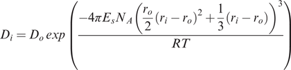
where
Di is the partition coefficient
Do is the strain-free partition coefficient, i.e., the partition coefficient for an ion the same size as that of the site and the same charge as i which enters the lattice without strain
Es is the effective Young’s modulus of the site (the elastic response to lattice strain). Blundy and Wood (1994) showed that elasticity varies linearly with the charge of the cation.
ro is the radius of the site
ri is the radius of ion i
R is the gas constant
T is temperature in Kelvin
Two tests of the lattice strain model demonstrate its utility. First, on a cation radius versus partition coefficient diagram of the type first pioneered by Onuma et al. (1968) and often known as an Onuma diagram, comparisons between measured partition coefficients and those calculated using the equation of Brice (1975) (Eq. 4.5) show very good agreement (Blundy and Wood, 1994) indicating that the model is appropriate for cations with a range of ionic charge in a number of different silicate phases (Figure 4.3). Second, the lattice strain model has a powerful predictive capability which allows partition coefficients to be calculated for elements where there are no experimental data from those whose values are already known. Blundy and Wood (1994) calculated partition coefficients for Ra in plagioclase and clinopyroxene at a time when these were not experimentally determined. Subsequent experimental studies found excellent agreement between the measured and calculated values.
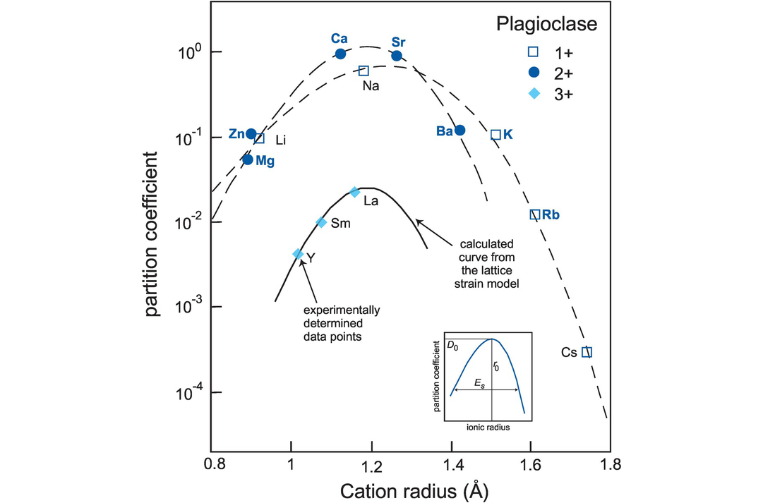
A plot of experimentally determined partition coefficients (expressed as log to the base 10) versus ionic radius (in angstroms: 10−10 m) for trace elements in plagioclase in equilibrium with silicate melt in the system diopside–albite–anorthite (after Wood and Blundy, 1997; adapted by permission of Springer-Nature). Diagrams of this type are known as Onuma diagrams. The curves drawn through the cations of equal valency are calculated from the lattice strain model (Eq. 4.5). The measured partition coefficients for mono-, di- and trivalent cations define separate parabolic curves which become tighter as the charge on the cation increases. This is due to the increase in the effect of Young’s modulus on the site with increasing charge. The peak of the parabola corresponds to the ‘best fit’ ionic radius ro and partition coefficient Do which is the optimum size of the site in plagioclase (see inset). Partition coefficients decrease as the size of the site deviates either positively or negatively from ro. Deviations from the anticipated parabolic pattern may reveal controls on trace element partitioning other than those of the size and charge of the cation. Onuma diagrams can also be used to estimate the size of a distribution coefficient when measurements have been made for a similar element. The inset diagram illustrates the three key parameters of the lattice strain model: ro, the radius of the site; Do, the strain-free partition coefficient; and Es, the elastic response of that site to lattice strain as measured by Young’s modulus.
Thermodynamic theory indicates that the lattice strain parameters (Do, ro and Es) are a function of key variables such as pressure, temperature and composition, and increasingly the trend is for the lattice strain parameters to be parameterised from a range of experimental studies. These equations can then be used to calculate partition coefficients for a specific set of conditions for a given group of trace elements. Wood and Blundy (1997) show how this methodology may be used to quantify partition coefficients for REE and Y in clinopyroxene and allows for the precise quantification of DREE during the polybaric fractional melting of the mantle.
4.2.1.3 Physical Controls on the Value of Partition Coefficients in Mineral-Melt Systems
Thus far we have shown how ionic size and charge are important parameters in the partitioning of trace elements between minerals and melt and how these properties may be quantified from experimental data. We have also noted that consideration of mineral-melt equilibria from a thermodynamic standpoint indicates that partitioning is also governed by properties such as melt composition, temperature and pressure. In the section that follows we illustrate empirically the effects of these and other intensive variables on the size of mineral-melt partition coefficients.
(a) Composition. Two very significant studies from the 1970s demonstrate that trace elements show distinct preferences when partitioned between immiscible acid and basic melts (Watson, 1976; Ryerson and Hess, 1978), indicating that melt composition exerts a major control on trace element partitioning. Typically, the values of partition coefficients are higher in more siliceous melts, sometimes by as much as an order of magnitude, as illustrated with respect to the partitioning of the REE between hornblende and basaltic, intermediate and felsic melts (Figure 4.4a).
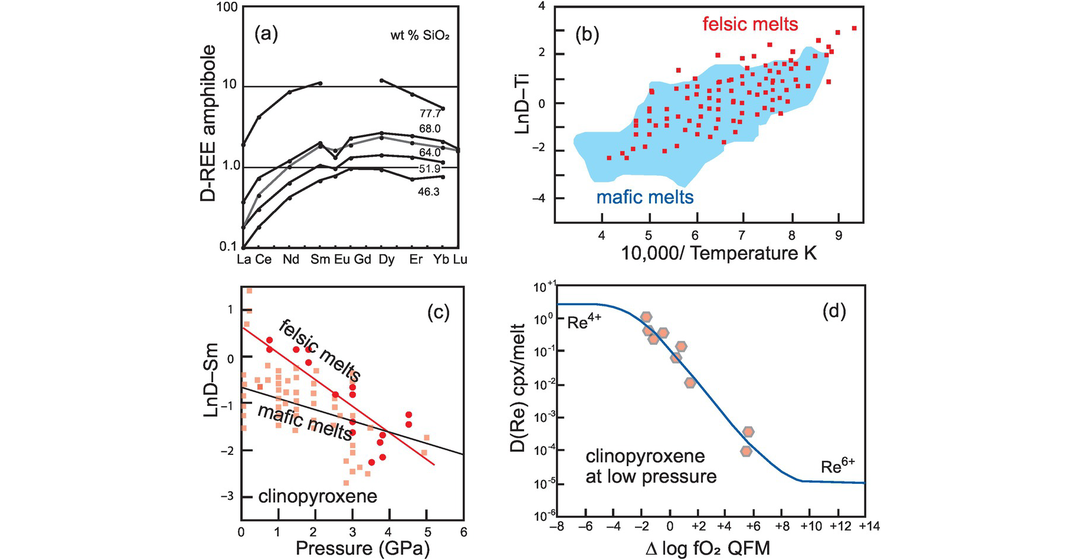
(a) Partition coefficients for REE between amphibole and silicate melt show an increase with increasing SiO2 content of the melt (data from Tiepolo et al., 2007). In mafic melts (low silica content) light REE are incompatible and middle and heavy REE are compatible. In felsic melts (high silica content) all the REE are compatible. (b) Variation in partition coefficient for Ti in clinopyroxene with temperature. LnD–Ti increases with falling temperature (increasing 10,000/K). Mafic melts are represented by the shaded field and felsic melts by squares (after Bédard, 2014; with permission from John Wiley & Sons). (c) Variation in partition coefficient for Sm in clinopyroxene with pressure. LnD–Sm decreases with increasing pressure. The solid red line and circular data points are for felsic melts, the grey line and square data points are for mafic melts (after Bédard, 2014; with permission from John Wiley and Sons). (d) Variation in partition coefficients for Re in clinopyroxene with changing oxygen fugacity. At high oxygen fugacities the dominant ion is Re4+ which is compatible. At low oxygen fugacities the dominant ion is Re6+, which is strongly incompatible.
Much of this compositional dependence is related to structural changes in the melt phase and the increased polymerisation of the more silica-rich melts. There are two commonly used models for describing the degree of structural organisation in a melt. There is the NBO/T notation in which the ratio of non-bridging oxygen (NBO) ions is expressed relative to the proportion of tetrahedrally coordinated cations (T) ions (Si and Al). It has been shown that with increasing melt polymerisation there is a decrease in NBO ions which leads to fewer sites available in the melt to accommodate trace elements such as the REE. This gives rise to higher partition coefficients for the REE. In contrast, partition coefficients for cations with a low charge/size ratio decrease with increasing melt polymerisation due to their coupled substitution with Al (Bennett et al., 2004). The parameter NBO/T can be calculated using the method of Mysen (1988) and varies between 4.0 for an unpolymerised melt to less than 1.0 for a 3D network. This notation has been used as a measure of melt composition in trace element partitioning studies by Schmidt et al. (2006).
A slightly different notation is the Xnf/X parameter where Xnf is the sum of the molar fraction of the network-forming (nf) cations (Si and some Al) normalised to X, the sum of all the cations calculated on a molar basis. This has been used to assess changes in melt structure in amphibole trace element partitioning experiments by Tiepolo et al. (2001, 2007).
In addition to the importance of the silica content of melts on the magnitude of trace element partition coefficients, other elements may also play an important role. Bennett et al. (2004) show that the Na content of a melt in the Na2O–CMAS system has an important effect on trace element partitioning between clinopyroxene and melt. In more sodic melts partition coefficients of the more highly charged (3+ and 4+) ions are higher by up to an order of magnitude relative to values in the ‘pure’ CMAS system. In addition, in some phases compositional controls on element partitioning may be exerted by ‘local’ crystal-chemical controls in specific mineral phases. Examples are given below in the mineral data for basalt partition coefficients (Section 4.2.1.5).
(b) Temperature. A good example of the control of temperature on partition coefficients comes from the compilation of experimental data by Bédard (2014) for calcic clinopyroxenes. These results show a strong negative correlation between 
(c) Pressure. One of the more convincing demonstrations of the effect of pressure on partition coefficients is the work of Green and Pearson (1983, 1986) on the partitioning of REE between sphene and an intermediate silicic liquid. Within a small compositional range (56–61 wt.% SiO2) at 1000°C they showed that there is a measurable increase in partition coefficient with increasing pressure from 7.5 to 30 kb. A more recent and petrologically important example is that of REE partitioning in clinopyroxene by Bédard (2014). He reviewed a voluminous amount of experimental data and showed that in both mafic and felsic melts DREE decreases with increasing pressure (illustrated with DSm in Figure 4.4c). Given that clinopyroxene is the principal host of REE in mantle rocks this observation has important implications for melting at different depths in the mantle. Similarly, some HFSE (notably Ti and Zr) show a similar property and in some amphiboles DTi,Zr decreases with increasing pressure (Dalpe and Baker, 2000).
(d) Oxygen fugacity and the importance of redox-sensitive trace elements. In experimental studies oxygen fugacity (fO2) is often buffered and this is normally reported relative to the quartz–fayalite–magnetite (QFM) oxygen buffer. fO2 values are a function of temperature, and so reference is sometimes made to the QFM fO2–T buffer curve. The QFM buffer tends to be used as a reference point since this is thought to approximate to the oxidation state of the upper mantle. However, in natural magmatic systems oxygen fugacity can vary by several orders of magnitude, and so the redox effect on trace element partitioning for heterovalent cations can be significant. Elements in this category include the first-row transition series elements, the PGE + Re and Eu, although experimental studies show that the most important redox-sensitive trace elements can be reduced to just V, Re, Eu and the major element Fe. As an example, the element Re may form the ions Re4+ and Re6+ in terrestrial magmas. As the Re ion becomes more oxidised there is a reduction in ionic size from 63 to 55 pm (10−12 m) (Shannon, 1976). This reduction in ionic size influences the partitioning of the element into specific sites in the mineral lattice. Mallmann and O’Neill (2007) showed that Re4+ is moderately compatible in garnet and clinopyroxene, slightly incompatible in orthopyroxene and spinel, and incompatible in olivine, but Re6+ is incompatible in all phases (Figure 4.4d). In a similar way the trace element V has the potential to form the ions V2+, V3+, V4+ and V5+ with the resultant reduction in ionic radius from 79 to 54 pm, for six-fold coordination, with increased oxidation (Shannon, 1976). Mallmann and O’Neill (2009) explored the change in the measured partition coefficients for DV during mantle melting over a wide range of redox conditions (−13 to +11 fO2 relative to the quartz–fayalite–magnetite oxygen buffer) – this covers the known redox conditions of the entire inner solar system. They showed that at low oxygen fugacity V is compatible in the phases olivine, pyroxene and spinel, whereas at high oxygen fugacity it is highly incompatible. The systematic change in partition coefficient with increasing oxygen fugacity for elements such V and Re means that their concentrations in basaltic melts will vary according to the redox conditions of mantle melting. These data have been inverted to calculate the redox state of the mantle in different tectonic settings (see Mallmann and O’Neill, 2007, 2009, 2013, 2014; Laubier et al., 2014).
The most redox-sensitive trace element in plagioclase is Eu. At low oxygen fugacities europium forms Eu2+ whereas at high fugacities it forms Eu3+ and the two species behave very differently in their partitioning between plagioclase and a basaltic melt, for the larger Eu2+ ion is more compatible than the smaller Eu3+ in plagioclase. Eu when divalent follows Sr, whereas the trivalent oxidised form follows the REE (Drake and Weill, 1975; Aigner-Torres et al., 2007). The net result of this is that the partitioning behaviour of Eu may depart from that of the other REE leading to an Eu anomaly in the REE pattern.
(e) Water content of the melt. The addition of water to a silicate melt has two opposing effects on partition coefficients. First, since the presence of water lowers the crystallisation temperature of a melt, this may cause partition coefficients to increase, but, second, the presence of water may the lower the activity and activity coefficients of the trace components in the melt such that partition coefficients may decrease (Wood and Blundy, 2014). Gaetani et al. (2003) found that during the partial melting of hydrous peridotite clinopyroxene REE partition coefficients were lower than predicted. They attributed this reduction in DREE to a change in the degree of melt polymerisation caused by the addition of water to the melt. In plagioclase Bédard (2006) noted that DTi and DREE increase as the water content of the melt increases.
4.2.1.4 Selecting an Appropriate Partition Coefficient
It is clear from the foregoing discussion that selecting an appropriate partition coefficient is not simple given the large number of variables to consider. A further complexity is the observation that mineral-melt partition coefficients are not constant during differentiation processes, for as a melt differentiates the composition of the melt, the pressure and the temperature will all change (Wood and Blundy, 2014). Sometimes the effects of the different variables can be inter-related, as, for example, when the liquidus temperature of a melt is a function of composition as in the case for olivine in a magnesian melt. At other times the effects of two different variables may cancel each other out. An example would be the contrasting effects of increased pressure, which serves to increase the partition coefficient, and increasing temperature, which reduces it.
Given the important control of melt composition on the size of partition coefficients, Nielsen and Drake (1979) and Neilsen and Dungan (1983) sought to minimise the impact of this variable by considering melt composition as a two-lattice melt model. In this model, the melt is assumed to be made up of two independent lattices comprising the network-forming and the network-modifying cations and anions. Partition coefficients are then parameterised against complex functions of melt chemistry. However, as Bédard (2005) pointed out there are some difficulties with this approach. First, some cations can fulfil multiple structural roles within the melt. In addition, the parameterisation of D-values requires that the melt composition be known exactly, and while this might work in laboratory experiments it cannot always be applied to natural rock samples.
Given that not all trace element data is adequately parameterised, a more empirical approach is taken here. Tables of partition coefficients (Tables 4.1–4.4) have been compiled from the literature to illustrate ‘indicative’ partition coefficients. It is recommended that these are used as a guide in petrological modelling and should not be taken as definitive. For a particular petrological model, partition coefficients should be taken from experimental studies that most closely match those of the conditions being modelled. The partition coefficients tabulated here are organised by melt composition and are drawn from the huge wealth of experimental work on trace element partitioning now published.
Much of the older partition coefficient (Kd) data is summarised in the GERM (Geochemical Earth Reference Model) database collated by R. Neilson at https://earthref.org/KDD/.https://earthref.org/GERM/tools/tep.htm. This database includes partition coefficients for a range of mineral species hosted in a wide range of rock types and has the advantage of being searchable, and the results can be downloaded into an Excel spreadsheet. In addition to individual experimental studies, there are some helpful syntheses such as the special volume of Lithos edited by Austreheim and Griffin (2000). In addition, compilations of partition coefficient data for specific minerals include olivine (Bédard, 2005), plagioclase (Bédard, 2006), orthopyroxene (Bédard, 2007), clinopyroxene (Bédard, 2014), and amphibole Tiepolo et al. (2007).
The longer-term aim of trace element partitioning studies is that all the relevant variables should be parameterised. This will include the composition of the mineral host, the composition of the melt, pressure and temperature. The extent to which this has already been accomplished is summarised in the review by Wood and Blundy (2014).
4.2.1.5 Partition Coefficients in Basalts
Some indicative partition coefficients for the geologically important trace elements in minerals in equilibrium with basaltic melts are listed in Table 4.1. The compilation is based upon a range of sources outlined below. Some REE values are interpolated, and those associated with some minerals common in mafic melts are shown in Figure 4.5. In the discussion that follows the relevant experimental conditions are included where possible. Averages are calculated as median values.
| Atomic number | Symbol | Name | Olivine | Orthopyroxene | Clinopyroxene | Garnet | Plagioclase | Ca-Amphibole |
|---|---|---|---|---|---|---|---|---|
| 3 | Li | Lithium | 0.198 | 0.200 | 0.200 | 0.022 | 0.2940 | 0.104 |
| 4 | Be | Beryllium | 0.248 | 0.016 | 0.047 | 0.003 | 0.5675 | 0.170 |
| 5 | B | Boron | 0.0055 | 0.018 | 0.036 | 0.0045 | 0.1860 | 0.010 |
| 19 | K | Potassium | 0.006845 | 0.0003 | 0.007 | 0.00061 | 0.2030 | 0.400 |
| 21 | Sc | Scandium | 0.1200 | 1.290 | 1.750 | 2.620 | 0.0160 | 4.940 |
| 22 | Ti | Titanium | 0.0096 | 0.759 | 0.380 | 0.290 | 0.0380 | 2.665 |
| 23 | V | Vanadium | 0.0896 | 0.856 | 2.900 | 3.600 | 0.0100 | 6.080 |
| 24 | Cr | Chromium | 1.180 | 3.520 | 8.100 | 2.010 | 0.0450 | 6.030 |
| 25 | Mn | Manganese | 1.632 | 1.410 | 0.895 | 0.865 | 0.0290 | nd |
| 27 | Co | Cobalt | 5.294 | 2.480 | 1.350 | 0.950 | 0.1490 | nd |
| 28 | Ni | Nickel | 24.010 | 7.380 | 2.600 | 5.100 | 0.1620 | nd |
| 29 | Cu | Copper | 0.1100 | nd | 0.360 | 0.575 | 0.1400 | nd |
| 30 | Zn | Zinc | 0.8300 | nd | 0.490 | 1.148 | 0.1300 | nd |
| 31 | Ga | Gallium | 0.1026 | 0.206 | 0.740 | 1.010 | 1.7000 | nd |
| 37 | Rb | Rubidium | 0.0007 | 0.003 | 0.010 | 0.0007 | 0.1140 | 0.090 |
| 38 | Sr | Strontium | 0.000138 | 0.0012 | 0.088 | 0.0074 | 1.6290 | 0.660 |
| 39 | Y | Yttrium | 0.007190 | 0.0950 | 0.670 | 8.5000 | 0.0371 | 1.325 |
| 40 | Zr | Zirconium | 0.008 | 0.0320 | 0.1115 | 0.7300 | 0.0010 | 0.370 |
| 41 | Nb | Niobium | 0.004 | 0.0013 | 0.0037 | 0.0055 | 0.0970 | 0.390 |
| 42 | Mo | Molybdenum | 0.1034 | 0.0039 | 0.014 | nd | nd | nd |
| 44 | Ru | Ruthenium | 1.0000 | nd | 2.400 | nd | nd | nd |
| 45 | Rh | Rhodium | 2.6960 | nd | 0.240 | nd | nd | nd |
| 46 | Pd | Palladium | 0.1000 | nd | < 0.3 | nd | nd | nd |
| 55 | Cs | Caesium | 0.0007 | nd | nd | nd | 0.5960 | 0.030 |
| 56 | Ba | Barium | 0.000023 | 0.000006 | 0.0002 | 0.00037 | 0.2470 | 0.385 |
| 57 | La | Lanthanum | 0.000022 | 0.0008 | 0.086 | 0.0047 | 0.1630 | 0.200 |
| 58 | Ce | Cerium | 0.000045 | 0.0016 | 0.175 | 0.0179 | 0.0960 | 0.350 |
| 59 | Pr | Praseodymium | 0.000085 | 0.0032 | 0.289 | 0.0593 | 0.1320 | 0.610 |
| 60 | Nd | Neodymium | 0.000200 | 0.0056 | 0.470 | 0.170 | 0.0908 | 0.730 |
| 62 | Sm | Samarium | 0.000636 | 0.0150 | 0.810 | 0.870 | 0.1060 | 1.075 |
| 63 | Eu | Europium | 0.001200 | 0.0300 | 1.000 | 1.630 | 0.1005 | 1.130 |
| 64 | Gd | Gadolinium | 0.001800 | 0.0340 | 1.040 | 2.550 | 0.0502 | 1.370 |
| 65 | Tb | Terbium | 0.002750 | 0.0540 | 1.220 | 4.200 | 0.0500 | 1.390 |
| 66 | Dy | Dysprosium | 0.004000 | 0.0770 | 1.400 | 6.200 | 0.0293 | 1.405 |
| 67 | Ho | Holmium | 0.006430 | 0.1000 | 1.350 | 8.200 | 0.0250 | 1.360 |
| 68 | Er | Erbium | 0.0110 | 0.1200 | 1.340 | 9.600 | 0.0181 | 1.275 |
| 69 | Tm | Thulium | 0.0140 | 0.17 | 1.380 | 11.100 | 0.0150 | 1.200 |
| 70 | Yb | Ytterbium | 0.0188 | 0.2200 | 1.420 | 12.600 | 0.0110 | 1.050 |
| 71 | Lu | Lutetium | 0.0280 | 0.2200 | 1.160 | 13.700 | 0.0093 | 0.850 |
| 72 | Hf | Hafnium | 0.0080 | 0.0600 | 0.383 | 0.480 | 0.0100 | 0.680 |
| 73 | Ta | Tantallum | 0.0300 | 0.0025 | 0.0239 | 0.0215 | 0.0750 | 0.335 |
| 75 | Re | Rhenium | 0.010 | 0.180 | 0.200 | 0.100 | nd | nd |
| 76 | Os | Osmium | 0.53437 | nd | 0.010 | nd | nd | nd |
| 77 | Ir | Iridium | 0.42619 | nd | nd | nd | nd | nd |
| 78 | Pt | Platinum | 0.05140 | nd | nd | nd | nd | nd |
| 79 | Au | Gold | 0.10000 | nd | nd | nd | nd | nd |
| 82 | Pb | Lead | 0.0013 | 0.0013 | 0.009 | 0.00034 | 1.5920 | 0.095 |
| 90 | Th | Thorium | 0.0018 | 0.00002 | 0.013 | 0.0015 | 0.3050 | 0.020 |
| 92 | U | Uranium | 0.0013 | 0.00004 | 0.006 | 0.0104 | 0.0107 | 0.010 |
Notes: nd, no data
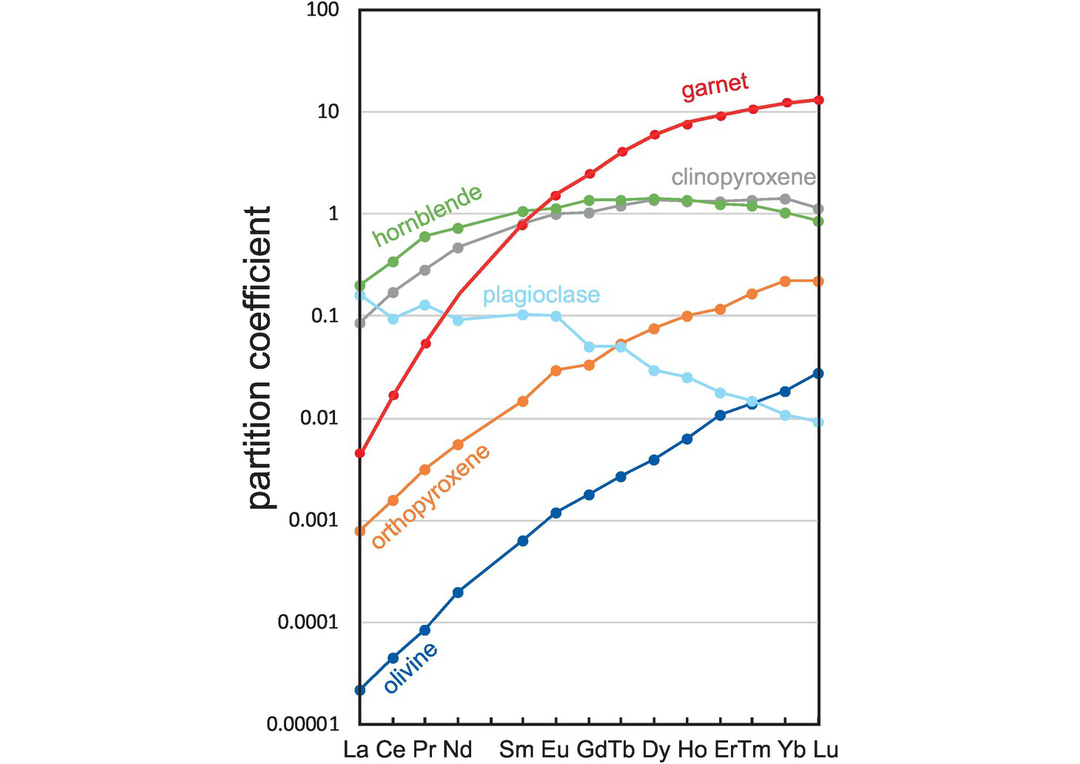
REE mineral-melt partition coefficients between the major silicate minerals and basaltic melts.
(a) Olivine. Most partition coefficients for trace elements in olivine vary with the MgO content of the melt and with temperature, for the two variables are strongly correlated. Many of these partition coefficients have been parameterised by Bédard (2005). For the highly siderophile elements partition coefficients tend to vary as a function of fO2 with an increase in Di as fO2 decreases (Righter et al., 2004). For the REE, partition coefficients increase with increasing Al in olivine and decrease with increasing pressure and with Fo content of the olivine (Sun and Liang, 2013).
Olivine–melt partition coefficients for Ti, V, Mn, Co and Ni are taken from the experimental study of Laubier et al. (2014) for MORB melts (MgO = 8.56 wt.%) using median values for experimental runs between 1150 and 1190°C, at 0.1 MPa (atmospheric pressure) and fO2= QFM. Values for K, Cs, Pb, Th, U, Zr, Nb, Hf and Ta are from the parameterisation of Bédard (2005) for melts with 11 wt.% MgO. Values for Li, Be, Cu, Mo and Ga are also from the compilation of Bédard (2005). Values for the REE, Y, Sc, Sr and Ba are from Beattie (1994) using the recommended results for a komatiitic melt (experiment C10) as most appropriate for partial melting calculations. This experiment was conducted at 1495°C, at atmospheric pressure and at log fO2 = −4.7. Partition coefficients for the HSE Ru, Pd, Re and Au are from the experimental study of Righter et al. (2004) on a Hawaiian ankaramite (MgO = 9.75 wt.%) at atmospheric pressure and 1300°C, adjusted for the oxygen fugacity of natural systems. Os, Ir and Pt are from the compilation of Bédard (2005). Zn and Cr are from the GERM database.
(b) Orthopyroxene. Partition coefficient data for orthopyroxene in a basaltic melt for the REE, HFSE and Sr are from the experimental study of Green et al. (2000). This study shows that partition coefficients in orthopyroxene are strongly influenced by the Al content of the orthopyroxene. Average values were taken from experiments on a tholeiitic basalt (Mg# = 59), conducted under hydrous conditions at 2.0–7.5 GPa and 1080–1200°C and a fO2 between the Ni–NiO and magnetite–wustite buffers. Partition coefficients for Sc, Ti, V (at QFM) and Mn, Co, Ni, Ga are from the average experimental values of Laubier et al. (2014) in a MORB melt (MgO = 8.56 wt.%) at 1150–1190°C, 0.1MPa and fO2 = QFM to NNO+2. Partition coefficients for B, Be and Li are from the experimental study of Brenan et al. (1998) on a basaltic andesite at 1000–1350°C at atmospheric pressure. Data for K, Rb and Ba are from the GERM database and Cr is for Cr3+ from Mallmann and O’Neill (2009), who show that chromium partition coefficients for orthopyroxene increase with increasing oxygen fugacity.
(c) Clinopyroxene. Bédard (2014) showed that there is significant crystal chemical control in trace element partitioning in clinopyroxene. For example, there is a positive correlation between DTi and the tetrahedral Al content of clinopyroxenes implying a coupled Ti–Al substitution. A similar pattern was observed for DZr and DCo which also increase with increasing alkali content and silica content but decrease with increasing Mg# and CaO content (Bédard, 2014).
Here partition coefficient data for clinopyroxenes for the REE, HFSE and Sr are from the experimental study of Green et al. (2000) conducted on a tholeiitic basalt (Mg# = 59), as described above for orthopyroxene. In these experiments both the water content and the temperature of the melt influence trace element partitioning, although the effect of water is greater than that of temperature such that partition coefficients are lower under hydrous conditions. Sr values are pressure-sensitive and DSr increases with increasing pressure. Partition coefficient values for the elements Mo, Ru, Rh and Pd are from the compilation of Bédard (2014) and Be, B, Sc, K, Ti, V, Cr, Mn, Ga, Rb, Re, Os, Pb, U and Th are from the GERM database; median values are used where there are multiple records.
(d) Garnet. Partition coefficient data for garnet for the REE, HFSE and Sr are from the experimental study of Green et al. (2000) on a tholeiitic basalt (Mg# = 59), as described above for orthopyroxene. As noted, both the water content and the temperature of the melt influence trace element partitioning such that at lower temperatures partition coefficients increase whereas under higher water contents partition coefficients decrease. Thus, the two effects tend to cancel each other out. Partition coefficients for Li and K are from the experimental study of Gaetani et al. (2003) on the melting of hydrous peridotite at 1.2 GPa and 1185°C. Partition coefficients for B, Be, Sc, Ti, V, Ni, Rb, Ba, Cr, Mn, Co, Ni, Zn, Ga, Pb, Th and U are from the GERM database. Re is reported as Re4+ at the conditions of the QFM buffer after Mallmann and O’Neill (2007).
(e) Plagioclase. Trace element partitioning between plagioclase and a basaltic melt is strongly dependent on the An content of the plagioclase and most partition coefficients increase with decreasing An content (Blundy and Wood, 1991; Bindeman et al., 1998; Bédard, 2006; Tepley et al., 2010). In addition, the partition coefficients of a small number of elements (Zr, Fe, Eu and Cr) are sensitive to fO2 (Aigner-Torres et al., 2007). There is no significant temperature control (Bindeman et al., 1998).
Partition coefficient data for plagioclase for the LILE, HFSE and first transition series elements were selected from the experimental database of Aigner-Torres et al. (2007) for the partitioning between plagioclase (An73–79) and MORB at 1200°C, atmospheric pressure and fO2 = QFM. Additional data for B, Be, V, Co, Ni, U and the REE + Y were obtained from the experimental studies of Bindeman et al. (1998) and Bindeman and Davis (2000). These experiments are for a basaltic andesite at T = 1426–1572 K, in air, at atmospheric pressure with plagioclase compositions between An75 to An77.2. Partition coefficients for Zn, Ga, Hf and Cu are from the GERM database.
(f) Amphibole. Trace element partitioning in amphibole is complex because of the number of different sites in the mineral lattice. There are three octahedral sites: M1, M2 and M3; an eight-fold M4 site occupied by Ca and Na; and a twelve-fold A-site occupied by Na and K or that may be vacant. The different sizes of these sites mean that they will exert different preferences for trace elements. Experimental studies show that partition coefficients in amphibole vary primarily as a function of the degree of melt polymerisation and are not strongly influenced by changes in P or T (Tiepolo et al., 2007). The effects of melt composition have been parameterised for the REE and Y as a function of Xnf/X (Tiepolo et al., 2007) (see Section 4.2.1.3). In addition, there are local crystal-chemical effects such as the Ca content (Wood and Blundy, 2014) and Mg# (Tiepolo et al., 2001), and for a few elements (Ti, Hf, Zr, Rb, Ba, La, Nd) oxygen fugacity also exerts a small effect (Dalpe and Baker, 2000).
The partition coefficient data listed here are for calcic-amphiboles and are from the review of Tiepolo et al. (2007). Experimental data were selected for melts in the range SiO2 = 48.1–52.4 wt.% at temperatures and pressures between 950 and 1070°C and 0.2–1.4 GPa and at fO2 = QFM − 2.
4.2.1.6 Partition Coefficients in Andesites
The partition coefficients for trace elements between rock-forming minerals and andesitic melts (57–63 wt.% SiO2 as defined in the TAS classification) are shown in Table 4.2 and Figure 4.6. This compilation is based upon the range of sources outlined below. Some REE values are interpolated. Where possible the relevant experimental conditions are included. Averages are calculated as median values. Some data are from the GERM database. Early compilations for mineral–andesite partition coefficients are based upon phenocryst–matrix studies but are highly variable (Luhr and Carmichael, 1980; Gill, 1981). This is, in part, due to the range of melt compositions examined, the presence of mineral inclusions in the mineral separates analysed and the precision of the analytical methods used.
| Atomic number | Symbol | Name | Olivine | Orthopyroxene | Clinopyroxene | Garnet | Plagioclase | Hornblende |
|---|---|---|---|---|---|---|---|---|
| 3 | Li | Lithium | 1.300 | 0.783 | nd | nd | 0.450 | 0.124 |
| 4 | Be | Beryllium | nd | 0.360 | nd | nd | 0.300 | nd |
| 19 | K | Potassium | nd | 0.014 | 0.011 | 0.010 | nd | nd |
| 21 | Sc | Scandium | 0.283 | 3.875 | 14.000 | 3.900 | nd | 10.550 |
| 22 | Ti | Titanium | 0.030 | nd | nd | 2.620 | 0.047 | 2.320 |
| 23 | V | Vanadium | 0.080 | 1.000 | 3.150 | 8.000 | 0.270 | 9.650 |
| 24 | Cr | Chromium | 5.3–34 | 21–143 | 30–245 | 22.000 | (0.075) | 1.59–60.5 |
| 25 | Mn | Manganese | nd | 7.300 | 4.500 | nd | nd | 0.680 |
| 27 | Co | Cobalt | 1.885 | 12.000 | 5.500 | 1.800 | nd | 1.77–6.1 |
| 28 | Ni | Nickel | 20.800 | 0.79–24 | 4.6–9 | 0.600 | nd | 10.000 |
| 29 | Cu | Copper | 2.200 | 0.190 | 0.660 | nd | nd | 11.600 |
| 30 | Zn | Zinc | 1.500 | 3.500 | 2.000 | nd | nd | 0.42–8.7 |
| 31 | Ga | Gallium | 0.250 | 0.320 | 0.470 | nd | nd | nd |
| 37 | Rb | Rubidium | 0.036 | 0.022 | 0.030 | 0.010 | 0.015 | 0.140 |
| 38 | Sr | Strontium | 0.020 | 0.005 | 0.280 | nd | 2.625 | 0.280 |
| 39 | Y | Yttrium | 0.045 | 0.343 | 2.000 | 11.000 | 0.024 | 2.500 |
| 40 | Zr | Zirconium | 0.010 | 0.031 | 0.290 | 0.530 | 0.001 | 0.260 |
| 41 | Nb | Niobium | 0.035 | 0.027 | 2.100 | 0.040 | 0.018 | 0.280 |
| 42 | Mo | Molybdenum | 0.111 | 1.323 | nd | nd | nd | nd |
| 55 | Cs | Caesium | 0.01–0.27 | 0.01–0.38 | 0.01–0.64 | nd | 0.038 | 0.01–0.5 |
| 56 | Ba | Barium | 0.020 | 0.115 | 0.068 | nd | 0.498 | 0.120 |
| 57 | La | Lanthanum | 0.008 | 0.002 | 0.099 | 0.028 | 0.119 | 0.120 |
| 58 | Ce | Cerium | 0.008 | 0.005 | 0.193 | 0.080 | 0.094 | 0.240 |
| 59 | Pr | Praseodymium | 0.010 | 0.005 | 0.290 | 0.130 | 0.072 | 0.420 |
| 60 | Nd | Neodymium | 0.011 | 0.019 | 0.420 | 0.222 | 0.065 | 0.630 |
| 62 | Sm | Samarium | 0.015 | 0.073 | 0.750 | 0.810 | 0.046 | 1.370 |
| 63 | Eu | Europium | 0.017 | 0.057 | 0.990 | 1.540 | 0.630 | 1.080 |
| 64 | Gd | Gadolinium | 0.016 | 0.140 | 0.910 | 4.590 | 0.040 | 1.490 |
| 65 | Tb | Terbium | 0.025 | 0.240 | 1.050 | 6.300 | 0.053 | 1.650 |
| 66 | Dy | Dysprosium | 0.031 | 0.260 | 1.200 | 9.000 | 0.025 | 1.770 |
| 67 | Ho | Holmium | 0.037 | 0.410 | 1.550 | 15.000 | 0.018 | 1.600 |
| 68 | Er | Erbium | 0.044 | 0.430 | 1.900 | 20.000 | 0.014 | 1.470 |
| 69 | Tm | Thulium | 0.071 | 0.645 | 1.400 | 22.000 | 0.012 | 1.300 |
| 70 | Yb | Ytterbium | 0.071 | 0.590 | 0.900 | 24.000 | 0.010 | 1.150 |
| 71 | Lu | Lutetium | 0.110 | 1.035 | 0.700 | 24.000 | 0.009 | 1.070 |
| 72 | Hf | Hafnium | 0.020 | 0.115 | 0.368 | 0.440 | nd | 0.430 |
| 73 | Ta | Tantallum | 0.065 | 0.049 | 0.430 | 0.080 | 0.069 | 0.270 |
| 82 | Pb | Lead | 0.014 | nd | 0.870 | nd | ≫ 0.012 | 0.120 |
| 90 | Th | Thorium | 0.039 | 0.010 | 0.100 | nd | > 0.012 | 0.017 |
| 92 | U | Uranium | 0.057 | 0.012 | nd | nd | 0.012 | 0.008 |
Notes: nd, no data; values in parentheses are uncertain.
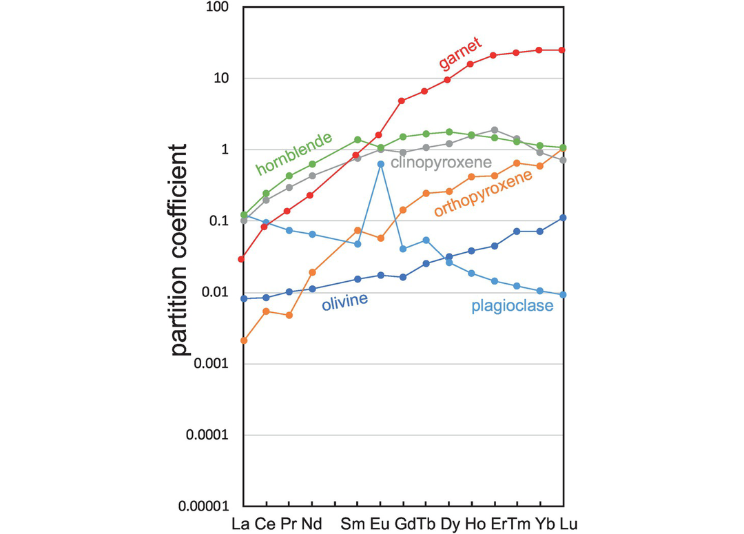
REE partition coefficients for the major silicate minerals in andesitic melts.
The olivine partition coefficients reported in Table 4.2 are from a single andesite (experimental melt compositions 56–60 wt.% SiO2) in Dunn and Sen (1994); Be, B and Li are from Brenan et al. (1998); and other data are from the GERM database. Similarly, the orthopyroxene data represent three andesite samples (experimental melt compositions 56–61 wt.% SiO2) from Dunn and Sen (1994) and the GERM database. The clinopyroxene REE and HFSE data are calculated from Klein et al. (2000) for a hydrous tonalitic melt (SiO2 = 57.9 wt.%) at 900–1000°C and 1.5–3.0 GPa, Be, B and Li from Brenan et al. (1998) and the GERM database. As in the case of basaltic melts clinopyroxene REE partition coefficients are composition-dependant and vary according to the jadeite content of the pyroxene. Experimental studies show that garnet REE partition coefficients are strongly temperature-dependent with partition coefficients increasing with decreasing temperature Klein et al. (2000). For this reason, garnet REE and HFSE partition coefficients are taken from a single hydrous experiment in the study of Klein et al. (2000) in which the temperature is 950°C and pressure 1.5 GPa. The hornblende REE and HFS partition coefficients are from Klein et al. (1997) for a melt composition with 57.9 wt.% SiO2; other data are from Brenan et al. (1995) and the GERM database. The partition coefficient data for plagioclase are averages from the four andesitic compositions studied by Dunn and Sen (1994) and from the GERM database, although, as already discussed, partition coefficients for plagioclase are in part a function of the An content of the plagioclase.
4.2.1.7 Partition Coefficients in Dacites and Rhyolites
Some indicative partition coefficients from published sources for the major rock-forming minerals in dacites, rhyodacites, rhyolites and high silica rhyolites are given in Table 4.3. These rocks have > 63 wt.%. SiO2 in the TAS classification. Compared with basaltic rocks, there are fewer modern experimental determinations of partition coefficient data for felsic rocks. Many published data sets are based upon phenocryst–matrix determinations and show some variability. In part this is because of the way partitioning behaviour is governed by melt structure and composition, but it also relates to other uncertainties with the matrix–phenocryst method discussed above. Data are drawn from a number of published sources supplemented with the compilations of Bacon and Druitt (1988) based upon rhyolites with 71 wt.% SiO2 and that of Nash and Crecraft (1985) for high-silica rhyolites (71–76 wt.% SiO2). The REE partition coefficients associated with some minerals common in felsic melts are shown in Figure 4.7.
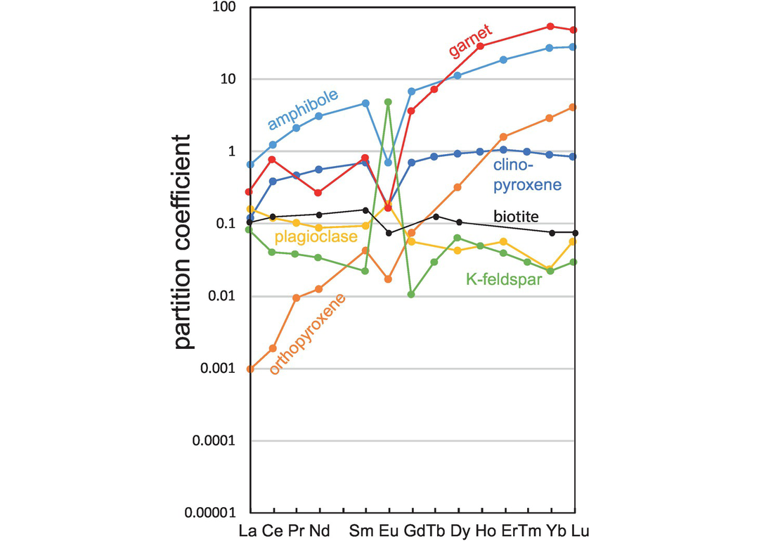
REE partition coefficients for the major silicate minerals in felsic melts.
| Atomic number | Symbol | Name | Orthopyroxene | Clinopyroxene | Garnet | Plagioclase | Amphibole | K-feldspar | Biotite | Ilmenite | Magnetite |
|---|---|---|---|---|---|---|---|---|---|---|---|
| 3 | Li | Lithium | 0.076 | 0.260 | nd | 0.152 | 0.700 | ||||
| 19 | K | Potassium | 0.004 | 0.002 | nd | nd | nd | nd | nd | nd | nd |
| 21 | Sc | Scandium | 7.100 | 15.900 | 20.200 | 0.010 | 11.790 | 0.027 | 4.9–20 | 5.9 | 5.000 |
| 22 | Ti | Titanium | 0.229 | 0.412 | 5.600 | 0.060 | nd | nd | nd | 150–235 | nd |
| 23 | V | Vanadium | nd | 7.440 | 7.000 | nd | 6.670 | nd | nd | nd | nd |
| 24 | Cr | Chromium | 10.000 | 30.000 | 3.850 | 0.100 | 40.000 | nd | 8.3–31 | 3.0000 | 30.000 |
| 25 | Mn | Manganese | 4.055 | 4.900 | nd | 0.060 | 3.890 | nd | 13.6–230 | 15–35 | 28–37 |
| 27 | Co | Cobalt | 38.000 | 17.000 | 3.000 | 0.150 | 37.000 | nd | nd | nd | 80.000 |
| 28 | Ni | Nickel | 11–25 | nd | nd | nd | 94.830 | nd | nd | nd | nd |
| 29 | Cu | Copper | nd | 0.110 | nd | 0.080 | 0.080 | nd | nd | nd | nd |
| 30 | Zn | Zinc | 6.000 | 1.960 | nd | 0.140 | 2.990 | nd | nd | 10.500 | 15.000 |
| 31 | Ga | Gallium | nd | 0.590 | nd | nd | 0.710 | nd | nd | nd | nd |
| 37 | Rb | Rubidium | nd | 0.030 | nd | 0.300 | 0.030 | 0.415 | 2.3–4.1 | nd | 0.010 |
| 38 | Sr | Strontium | 0.008 | 0.230 | 0.020 | 31.000 | 6.595 | 5.900 | 0.541 | nd | 0.010 |
| 39 | Y | Yttrium | 0.215 | 3.510 | 130.000 | 0.016 | 5.670 | nd | 1–1.4 | 0.2–1.6 | nd |
| 40 | Zr | Zirconium | 0.009 | 0.210 | 0.400 | 0.0002 | 0.450 | 0.195 | 1.3 | nd | 0.240 |
| 41 | Nb | Niobium | 0.002 | 0.210 | nd | 0.0025 | 1.400 | nd | 4–9.5 | 50.9–64.2 | nd |
| 42 | Mo | Molybdenum | nd | nd | nd | nd | 0.030 | nd | 1.7–5.7 | 3.000 | 6–16 |
| 55 | Cs | Caesium | 0.010 | 0.023 | nd | 0.030 | 0.100 | 0.123 | 1.2–4.4 | nd | 0.010 |
| 56 | Ba | Barium | 0.0007 | 0.010 | nd | 0.200 | 0.200 | 14.450 | 18 | nd | 0.100 |
| 57 | La | Lanthanum | 0.001 | 0.130 | 0.278–0.54 | 0.170 | 0.710 | 0.085 | 0.76–15.1 | 7.100 | 0.660 |
| 58 | Ce | Cerium | 0.002 | 0.410 | 0.79–0.93 | 0.130 | 1.350 | 0.042 | 0.86–11 | 7.800 | 0.710 |
| 59 | Pr | Praseodymium | 0.010 | 0.500 | nd | 0.110 | 2.300 | 0.039 | nd | nd | nd |
| 60 | Nd | Neodymium | 0.013 | 0.600 | 0.27–0.73 | 0.094 | 3.280 | 0.035 | 0.9–5.7 | 7.600 | 0.930 |
| 62 | Sm | Samarium | 0.045 | 0.760 | 0.84–1.04 | 0.100 | 4.950 | 0.023 | 1–4.3 | 6.900 | 1.200 |
| 63 | Eu | Europium | 0.018 | 0.190 | 0.167–0.31 | 0.200 | 0.750 | 4.900 | 0.59–4.7 | 2.500 | 0.910 |
| 64 | Gd | Gadolinium | 0.080 | 0.760 | 3.7–5.3 | 0.060 | 7.400 | 0.011 | nd | nd | nd |
| 65 | Tb | Terbium | nd | 0.900 | 7.2–11.9 | nd | nd | 0.030 | 0.87–3.9 | 6.500 | 1.300 |
| 66 | Dy | Dysprosium | 0.345 | 1.000 | nd | 0.045 | 12.165 | 0.065 | 0.76–3.4 | 4.900 | 1.6–4.4 |
| 67 | Ho | Holmium | nd | 1.070 | 28.2–34.5 | nd | nd | 0.050 | nd | nd | nd |
| 68 | Er | Erbium | 1.700 | 1.150 | nd | 0.060 | 20.000 | 0.040 | nd | nd | nd |
| 69 | Tm | Thulium | nd | 1.050 | nd | nd | nd | 0.030 | nd | nd | nd |
| 70 | Yb | Ytterbium | 3.150 | 0.960 | 54–67 | 0.025 | 29.465 | 0.023 | 0.6–3 | 4.100 | 0.440 |
| 71 | Lu | Lutetium | 4.400 | 0.900 | 47–64 | 0.060 | 30.000 | 0.030 | 0.6–3.4 | 3.600 | 0.300 |
| 72 | Hf | Hafnium | 0.054 | 1.410 | nd | 0.050 | 0.855 | nd | 0.44–0.84 | 3.100 | 0.240 |
| 73 | Ta | Tantallum | 0.110 | 0.500 | nd | 0.030 | 0.430 | 0.011 | 1.2–1.9 | 64–85 | 1.200 |
| 82 | Pb | Lead | 0.018 | 0.020 | nd | 0.180 | nd | 1.825 | 0.1–1.6 | nd | nd |
| 90 | Th | Thorium | 0.140 | 0.100 | nd | 0.010 | 0.160 | 0.220 | 0.27–2 | 7.500 | 0.010 |
| 92 | U | Uranium | nd | nd | nd | nd | nd | 0.048 | 0.46–1.2 | 3.200 | 0.21–0.83 |
Notes: nd, no data
Plagioclase partition coefficients for Li, Sr, Y, Zr, Nb, Ba, Hf and the REE are from Brophy et al. (2011). In this study phenocrysts in equilibrium with a rhyolitic partial melt in gabbro (SiO2 = 72–73 wt.%) were analysed by ion microprobe. The partition coefficients reported are median values of multiple analyses. Data for the elements Ti, Mn, Zn, Cu and Pb are from the experimental study of Iveson et al. (2018) conducted at 810–860°C, 1.5–4.05 kb and oxygen fugacity NNO = −0.5 to +2 log units. Melt compositions have 73–75 wt.% SiO2 (dry) and the plagioclase is An39–59. Other values are from Bacon and Druitt (1988). It has already been noted that trace element partition coefficients for plagioclase are strongly dependent on the composition of the host mineral and on melt temperature (Sun et al., 2017). In particular, there is a strong relationship between the partition coefficients for Sr and Ba and the mole fraction of anorthite in plagioclase. Both elements are more compatible in albite than in anorthite (Blundy and Wood, 1991).
Partition coefficient data for K-feldspar are from the GERM database. REE values are based upon average values and the missing values estimated by interpolation. Partition coefficient data for more sodic alkali feldspars are given by Streck and Grunder (1997) for the trace elements Cr, Mn, Co, Rb, Sr, Cs, Ba, REE, Hf, Ta and Th and by Wolff and Ramos (2014) for Rb, Cs, Sr, Ba and Pb.
Trace element partition coefficients for clinopyroxene are taken from the experimental study of Huang et al. (2006) for Cs, La, Ce, Sm, Eu, Er and Yb, with the remaining REE interpolated. In this study the silica content of the melt was ca. 69 wt.%. Data for Li, Sc, V, Mn, Zn, Ga, Cu, Sr, Y, Zr, Nb, Ba, Hf and Pb are from the more siliceous melts in the experimental study of Iveson et al. (2018). K and Ti are from the Severs et al. (2009) phenocryst–melt inclusion data for dacitic melts (SiO2 = 65 wt.%). The remaining elements are from Bacon and Druitt (1988) and from the GERM database.
Partition coefficient data for orthopyroxene for Li, Sr, Y, Zr, Nb, Ba, Hf and REE are from Brophy et al. (2011), with data for K, Ti and Pb from Severs et al. (2009) and for Ni from Stimac and Hickmott (1994). Other trace elements are from Bacon and Druitt (1988). It should be noted that there is considerable variation in some published trace element partition coefficients between orthopyroxene and felsic melts – compare, for example, the REE in the compilation of Bacon and Druitt with the study of Brophy et al. (2011), where the differences between these two studies may reflect the different silica content of the melts.
Trace element partition coefficients for amphibole for Li, Sr, Y, Zr, Nb, Ba, Hf and the REE are from Brophy et al. (2011), and for the elements Sc, V, Mn, Ni, Cu, Zn, Ga, Rb, Mo and Pb from Iveson et al. (2018). There are some differences between these and other published data, in particular for Rb, Sr, Zr, Ba, Mo and Pb, and again it appears that small differences in melt composition may induce significant variations in partition coefficient values. Other data are from Bacon and Druitt (1988).
Garnet partition coefficient data are from the GERM database where the REE data are based upon the phenocryst–matrix data of Irving and Frey (1978). Biotite partition coefficients also from the GERM database and are mostly phenocryst–matrix measurements taken from Nash and Crecraft (1985). Partition coefficient data for magnetite are from the compilation of Nash and Crecraft (1985) and Bacon and Druitt (1988). Ilmenite data are from the GERM database with the REE from Nash and Crecraft (1985), and values for Ti, Mn, Y, Zr and Ta are from the study of Stimac and Hickmott (1994) in which the melt composition was ~75 wt.% SiO2.
4.2.1.8 Partition Coefficients in Accessory Minerals
The minerals zircon, monazite, apatite, titanite and allanite occur primarily as accessory phases in felsic melts. These minerals occupy only a small volume of their parent rock but exercise a disproportionate effect on the distribution of some trace elements, in particular the REE. Further, they contain elements which are normally regarded as trace elements, but in these particular phases form a stoichiometric component of the host mineral. This means that they do not obey Henry’s law (Section 4.2.1) and therefore do not behave in the same way as other trace elements (Prowatke and Klemme, 2006; Chapman et al., 2016).
The appearance of an accessory phase in a melt is governed by the solubility of the phase in the melt. For example, in the case of zircon (ZrSiO4) the crystallisation of the mineral from a melt is governed by the solubility of Zr in the melt, such that when the melt is saturated in Zr, zircon will crystallise from the melt. In practice, therefore, zircon (and other accessory minerals) will appear in an igneous sequence towards the end of a differentiation process. Zr solubility is controlled by variables such as melt composition and temperature. Formulations of accessory mineral solubility have been given by Kelsey et al. (2008) for zircon and monazite, by Stepanov et al. (2012) for monazite, and by Harrison and Watson (1984) for apatite.
In this section the main focus is on the partition coefficients for the REE and for element pairs such as Nb–Ta and Th–U where either large partition coefficients or, in the case of element pairs, very different partition coefficients between the pair may have a major impact on the trace element composition of the melt. Partition coefficients for other elements derived from older mineral–matrix measurements are given in the GERM database. Relevant values are summarised in Table 4.4 and a plot of partition coefficients for the REE in accessory phases is given in Figure 4.8.
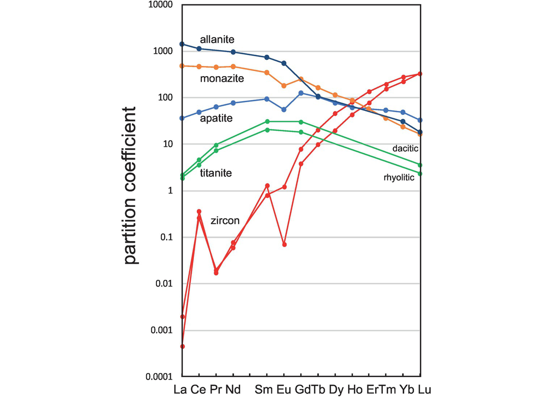
Partition coefficients for the REE in accessory minerals in felsic rocks (data from Table 4.4). Note the difference in scale from Figures 4.5–4.7.
Zircon (ZrSiO4) is one of the best studied accessory minerals because of its importance in geochronology and its use, when found as detrital grains in sediment, for recovering information about ancient continental crust. Hanchar and van Westrenen (2007) review the REE partition coefficient data for zircon and show that many of the published values in the older literature determined using phenocryst–matrix methods do not conform to the lattice strain model and are probably in error. This is particularly true for the incompatible light REE. They recommend the values of Sano et al. (2002) for zircon in equilibrium with a dacitic melt, and these are given in Table 4.4. A more recent study by Chapman et al. (2016) calculated trace element partition coefficients for a suite of bulk rock compositions from the Coast Mountains Batholith in British Columbia with SiO2 = 51–76 wt.%. The median values calculated for this suite are given in Table 4.4. An accurate measure of REE partition coefficients in zircon is particularly important when the partition coefficient data are inverted to estimate the parental melt composition as in the case of detrital zircons whose origin is unknown. The Chapman et al. (2016) partition coefficients seem robust in this respect. Trace element data for Y and Nb are from Chapman et al. (2016) and for B, Ti, Rb, Sr and Ba from Thomas et al. (2002). Ti concentrations in zircon may be used as a geothermometer (Watson et al., 2006) although Schiller and Finger (2019) give a more recent evaluation of the applicability of this methodology.
| Atomic number | Symbol | Name | Zircon | Apatite | Monazite | Titanite | Allanite | |||||||||
|---|---|---|---|---|---|---|---|---|---|---|---|---|---|---|---|---|
| Ref | 1 | 2, 3 | 1 | 4 | 5 | 5 | 6 | 6 | 7, 8 | 7, 8 | ||||||
| range | median | Dacite | Rhyolite | range | median | |||||||||||
| 3 | Li | Lithium | nd | nd | nd | 0.005 | nd | nd | nd | nd | nd | nd | ||||
| 5 | B | Boron | nd | 0.017 | nd | nd | nd | nd | nd | nd | nd | nd | ||||
| 22 | Ti | Titanium | nd | 3.150 | nd | nd | nd | nd | nd | nd | 1.94–4.03 | 2.675 | ||||
| 37 | Rb | Rubidium | nd | 0.006 | nd | nd | nd | nd | 0.00026 | 0.00033 | nd | nd | ||||
| 38 | Sr | Strontium | nd | 0.034 | nd | 24.000 | nd | nd | 0.62 | 0.44 | nd | nd | ||||
| 39 | Y | Yttrium | nd | 47.000 | nd | 24.000 | 20–606 | 78.500 | 14.3 | 8.96 | nd | nd | ||||
| 40 | Zr | Zirconium | nd | nd | nd | 0.012 | nd | nd | 3.78 | 3.48 | nd | nd | ||||
| 41 | Nb | Niobium | nd | 0.150 | nd | 0.009 | nd | nd | 7.26 | 5.44 | nd | nd | ||||
| 55 | Cs | Caesium | nd | nd | nd | nd | nd | nd | 0.0023 | 0.0022 | nd | nd | ||||
| 56 | Ba | Barium | nd | 0.004 | nd | 0.010 | nd | nd | 0.0025 | 0.0029 | nd | nd | ||||
| 57 | La | Lanthanum | 0.00046 | 0.002 | 36.0 | 24.0 | 74–3240 | 485.0 | 2.17 | 1.88 | 775–2819 | 1399 | ||||
| 58 | Ce | Cerium | 0.360 | 0.260 | 48.0 | 47.0 | 66–3011 | 459.5 | 4.6 | 3.61 | 628–2245 | 1120 | ||||
| 59 | Pr | Praseodymium | 0.017 | 0.020 | 64.0 | 34.0 | 71–3194 | 446.0 | 9.7 | 7.39 | nd | nd | ||||
| 60 | Nd | Neodymium | 0.077 | 0.060 | 77.0 | 36.0 | 73–3125 | 463.0 | nd | nd | 538–1980 | 970 | ||||
| 62 | Sm | Samarium | 0.800 | 1.300 | 93.0 | 42.0 | 56–2526 | 344.0 | 31.2 | 20.4 | 272–1254 | 728 | ||||
| 63 | Eu | Europium | 1.220 | 0.070 | 55.0 | 8.0 | 12–1759 | 177.5 | nd | nd | 138–794 | 549 | ||||
| 64 | Gd | Gadolinium | 8.000 | 3.800 | 127.0 | 45.0 | 49–1920 | 252.0 | 30.5 | 18.2 | nd | nd | ||||
| 65 | Tb | Terbium | 20.700 | 9.900 | 102.0 | nd | 34–1400 | 163.5 | nd | nd | 107–139 | 108 | ||||
| 66 | Dy | Dysprosium | 45.900 | 20.000 | 76.0 | 46.0 | 27–1015 | 115.5 | nd | nd | nd | nd | ||||
| 67 | Ho | Holmium | 80.000 | 44.000 | 62.0 | nd | 20–709 | 86.5 | nd | nd | nd | nd | ||||
| 68 | Er | Erbium | 136.000 | 77.000 | 57.0 | 88.0 | 16–534 | 57.5 | nd | nd | nd | nd | ||||
| 69 | Tm | Thulium | 197.000 | 154.000 | 53.0 | nd | 12–324 | 36.0 | nd | nd | nd | nd | ||||
| 70 | Yb | Ytterbium | 277.000 | 219.000 | 48.0 | 95.0 | 10–237 | 23.5 | nd | nd | 19–36 | 31 | ||||
| 71 | Lu | Lutetium | 325.000 | 331.000 | 33.0 | 91.0 | 8–187 | 16.5 | 3.65 | 2.38 | 12–23 | 18 | ||||
| 72 | Hf | Hafnium | nd | nd | nd | nd | nd | nd | 6.9 | 4.9 | nd | nd | ||||
| 73 | Ta | Tantallum | nd | nd | nd | nd | nd | nd | 84 | 54.8 | nd | nd | ||||
| 82 | Pb | Lead | nd | nd | nd | nd | nd | nd | 0.87 | 0.750000 | nd | nd | ||||
| 90 | Th | Thorium | nd | nd | nd | nd | 86–3853 | 691.000 | 0.14 | 0.101000 | 416–1331 | 732 | ||||
| 92 | U | Uranium | nd | nd | nd | nd | 9–377 | 60.000 | 0.07 | 0.090000 | 22–97 | 53 | ||||
Partition coefficient data for the REE in apatite (Ca5(PO4)3(F, Cl, OH)) given in Table 4.4 are from the ion microprobe study of Sano et al. (2002) for apatite in equilibrium with a dacitic melt and from Brophy et al. (2011) for apatite in contact with natural interstitial rhyolitic (71–76% SiO2) glass. Median values are given for the Brophy et al. (2011) REE partition coefficients, for these show a wide range of measured values and are higher than the Sano et al. (2002) data for the heavy REE.
Monazite ((LREE)PO4) is a light REE phosphate, xenotime mirror monazite ((Y,HREE)PO4) is its rarer heavy REE counterpart, and these phases are important in controlling REE concentrations during the melting and fractionation of crustal rocks. Stepanov et al. (2012) present partition coefficient data for Y, REE, Th and U in monazite. These partition coefficients were experimentally determined over a temperature range of 750–1200°C and a pressure range of 1–5 GPa on a hydrous Fe-, Mg-free peraluminous granitic melt with 76–78 wt.% SiO2. Partition coefficient values vary by over an order of magnitude, and the ratio of D-values for heavy to light REE increases with temperature and decreases with the water content of the melt. For this reason, the range of experimentally determined values and a median value are given in Table 4.4.
Selected trace element partition coefficients have been experimentally determined for titanite (sphene, CaTiSiO5) by Prowatke and Klemme (2005), who show that partition coefficients are strongly dependent upon melt composition. For this reason, values for both dacite (SiO2 = 64.3 wt.%) and rhyolite (SiO2 = 69.8 wt.%) are given in Table 4.4.
Klimm et al. (2008) give partition coefficients for allanite, a REE-rich member of the epidote group (Ca, (REE)Al2Fe2+(Si2O7)(SiO4)O(OH)), in felsic melts with between 71 and 74 wt.% SiO2 produced during the water-saturated melting of basalt. Their results for La, Ce, Nd, Sm and Eu, given as a range in Table 4.4, show that the partition coefficients are strongly temperature-dependant and decrease from 900 to 800°C. Partition coefficients for Tb, Yb and Lu are from Chesner and Ettlinger (1989).
4.2.2 Geological Controls on the Distribution of Trace Elements
The geochemical study of trace elements is a powerful tool for understanding and recognising geological processes. Our knowledge of the partitioning of trace elements between minerals and their parental melt means that a range of geological processes in which minerals are in equilibrium with a melt can be modelled. Further, inverting the modelling means that processes operating in a particular magmatic system may be identified. In contrast to magmatic systems, however, our knowledge of the behaviour of trace elements in aqueous and sedimentary systems is less amenable to quantification, and the main focus of this discussion is therefore upon magmatic systems. In this section we consider a range of geological processes for which there are quantitative models to describe the behaviour of trace elements. The relevant equations are given and the terms used are defined (Table 4.5). The interested reader will find a full derivation of the relevant equations in the text by Shaw (2006).
| Term | Definition |
|---|---|
| CA | Concentration of a trace element in the wall rock being assimilated during AFC processes |
| CL | Weight concentration of a trace element in the liquid |
 | Average weight concentration of a trace element in a mixed melt |
| CO | In partial melting the weight concentration of a trace element in the original unmelted solid; in fractional crystallisation the weight concentration in the parental liquid |
| Ck | Weight concentration of a trace element in the residual solid during crystal fractionation |
| CS | Weight concentration of a trace element in the residual solid (after melt extraction) |
| SSCB | Weight concentration of a trace element in a steady state liquid after a large number of RTF cycles |
| DO | Bulk distribution coefficient of the original solids |
| Dl | Mineral-melt partition coefficient, or the bulk distribution coefficient of the fractionating assemblage, during crystal fractionation |
| DS | Strain-free partition coefficient in the lattice strain model |
| DRS | Bulk distribution coefficient of the residual solids |
| F | Weight fraction of melt produced in partial melting; in fractional crystallisation the fraction of melt remaining |
| f | Fraction of melt allocated to the solidification zone in in situ crystallisation which is returned to the magma chamber |
| f' | A function of F, the fraction of melt remaining in AFC processes |
| ML | Mass of the liquid remaining during in situ crystallisation |
| MO | Total mass of the magma chamber in in situ crystallisation |
| n | Number of rock volumes processed during zone refining |
| P | Bulk distribution coefficient of minerals which contribute to a melt |
| r | Ratio of the assimilation rate to the fractionation rate in AFC processes |
| x | In an RTF magma chamber, the mass fraction of the liquid crystallised in each RTF cycle; during in situ crystallisation, the proportion of trapped melt in the magma chamber |
| y | Mass fraction of the liquid escaping in each RTF cycle |
4.2.2.1 Element Mobility
Any suite of rocks which has been affected by hydrothermal alteration or metamorphism is likely to have experienced some level of element mobility. It is essential, therefore, in any trace element study to first demonstrate that element concentrations are undisturbed and original before inferences can be made about the petrogenesis of the rock group. As was noted in Section 3.1.2, element mobility is controlled by the mineralogical changes which take place during alteration and the composition, temperature and relative volume of the migrating fluid or melt phase. Trace element mobility may be detected from mineralogical phase and compositional changes that have taken place in a rock as a result of metamorphism or hydrothermal activity, and careful petrography is an important tool in identifying chemically altered rocks. In addition, scattered trends on variation diagrams or divergent irregular patterns on multi-element plots (Section 4.4) are also useful indicators.
As a generalisation, incompatible elements which belong to the low field strength LILE group (Cs, Rb, K, Ba, Sr, ± Eu, and Pb) (Figure 4.2) are fluid-mobile, whereas the high field strength elements (the REE, Sc, Y, Th, Zr, Hf, Ti, Nb, Ta and P) are immobile (Pearce, 1983). Such generalisations are normally valid, but should not be assumed. For example, Humphries (1984) found that there is no simple relationship between the degree of mobility of the traditionally immobile REE and rock type, emphasising the importance of localised mineralogical and fluid controls. Humphries (1984) showed that the REE may be more easily released from a glassy basalt during alteration than from a rock with the same composition which is crystalline and that the REE may be mobilised by halogen-rich or carbonate-rich mineralising fluids in a rock in which they would otherwise be stable in the presence of an aqueous fluid.
4.2.2.2 Partial Melting
Melting in the Earth’s mantle typically takes place through the upwelling of hot mantle material and melting through decompression. For example, at a mid-ocean ridge hot mantle rises adiabatically, that is, without loss of heat by conduction, and progressively melts as it rises to the surface. Melting takes place at grain boundaries and is normally incomplete – hence the term ‘partial’ melting. For this reason, two important parameters must be considered in modelling partial melting processes. First is the nature of what is melting: the minerals involved in the melting process. The involvement of particular mineral phases at any stage in a particular partial melting event may be described with a melting reaction that is determined either experimentally or through petrographic observation. The phases included in the melting reaction are those which will govern the bulk partition coefficient of the melting process. The second key parameter is the extent of melting, or the melt fraction. This process is limited by the ability of the melt to ‘escape’ from its unmelted environment. This in turn is governed by the properties of both the melt and the host, in particular, the viscosity of the melt and the shape of the mineralogical network of the host.
Two types of partial melting process are commonly described in the geological literature and represent end-member models of natural processes. Batch melting, also known as equilibrium fusion and equilibrium partial melting, describes the formation of a partial melt in which the melt is continually reacting and re-equilibrating with the solid residue at the site of melting until mechanical conditions allow it to escape as a single ‘batch’ of magma. In fractional melting, also known as Rayleigh melting, only a small amount of liquid is produced before it is instantly isolated from the source. In this case, equilibrium is achieved only between the surface of the mineral grains in the source region.
Which partial melting process is appropriate in a particular situation depends upon the ability of a magma to segregate from its source region, which in turn depends upon the permeability threshold of the source. The problem is discussed in some detail by Wilson (1989). Fractional melting may be an appropriate model for some basaltic melts, as physical models of melt extraction from the mantle indicate that very small melt fractions can be removed from their source region (McKenzie, 1985; O’Nions and McKenzie, 1988). More viscous, felsic melts have a higher permeability threshold and probably behave according to the batch melting equation. It is important to note that physical models of melt extraction describe melt fractions in terms of their volume, whereas the chemical models used here more usefully describe melt fractions in terms of their mass.
(a) Batch melting. The concentration of a trace element in the melt CL is related to its concentration in the unmelted source Co by the expression
and the concentration of a trace element in the unmelted residue CS relative to the unmelted source Co is
where DRS is the bulk partition coefficient of the residual solid (see Eq. 4.4) and F is the weight fraction of melt produced. It should be noted that the bulk partition coefficient is calculated for the residual solids present at the instant the liquid is removed, so that solid phases that were present but are consumed during melting do not influence the trace element concentration in the liquid (Hanson, 1978). This formulation of the batch melting equation is very straightforward to use.
Modelling trace element behaviour during partial melting depends upon whether or not the minerals in the source rock contribute to the melt in their modal proportions. In the case of modal melting (where the minerals contribute to the melt in proportion to their concentration in the rock), the ratio of a trace element in the melt and the unmelted residue relative to the source is given by Eqs. 4.6 and 4.7. If, however, the phases in the host rock do not contribute to the melt in their modal proportions, then the batch melting equation for non-modal melting is expressed in terms of the original mineralogy of the source and the relative contributions each phase makes to the melt as determined from the melting reaction. In this case the equation for the melt is
where Do is the bulk distribution coefficient at the onset of melting and P is the bulk distribution coefficient of the minerals which are contributing to the melt. P is calculated from
where p1 is the weight normative fraction of mineral 1 in the melt and D1 is the mineral-melt distribution coefficient for a given trace element for mineral 1. Shaw (2006) illustrates the way in which the results of non-modal melting diverge from modal melting for elements with different compatibilities. His results indicate that for compatible elements at low degrees of melting (up to 10%) the two models give very similar results, whereas for incompatible elements the two models diverge after about 6–7% melting. More complex formulations which allow a phase to be consumed during melting, melt proportions to vary during partial melting, and variations in partition coefficients are given by Hertogen and Gijbels (1976) and Apted and Roy (1981).
Taking the most simple case where D is calculated for the unmelted residue (DRS, Eq. 4.6), the degree of enrichment or depletion relative to the original liquid (CL/Co) for different values of F can be determined for different values of DRS, the bulk distribution coefficient (Figure 4.9a). When DRS is small, Eq. 4.6 reduces to 1/F and marks the limit to trace element enrichment for any given degree of batch melting (effectively, the area to the right of D = 0.01 in Figure 4.9a). When F is small, Eq. 4.6 reduces to 1/D and marks the maximum possible enrichment of an incompatible element and the maximum depletion of a compatible element relative to the original source. It can be seen from this plot that at small degrees of melting the degree of enrichment or depletion varies hugely between compatible elements which are not enriched in the melt and incompatible elements which are strongly enriched in the melt. Thus, during batch melting incompatible/compatible element ratios are very sensitive at small degrees of melting. Enrichment and depletion in the solid residue in equilibrium with the melt (Eq. 4.7) for different values of F and D is shown in Figure 4.9b. Even small degrees of melting will deplete the residue significantly in incompatible elements, whereas compatible elements remain very close to their initial concentrations.
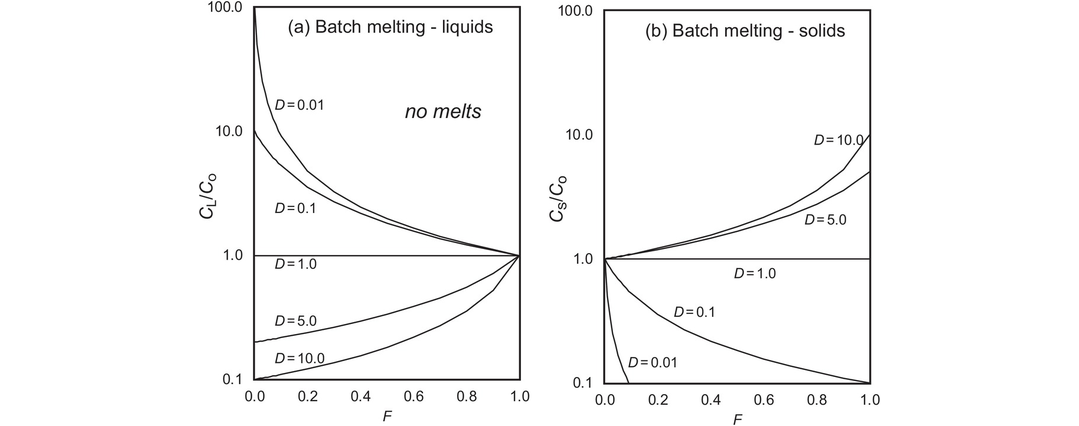
The enrichment of a trace element in a melt relative to its source (CL/Co) as a function of the fraction of melting (F), during modal batch melting for different values of bulk partition coefficient (D). (a) Relative concentrations in the melt fraction during modal batch melting. (b) Relative concentrations in the unmelted solid residue during modal batch melting.
(b) Fractional melting. In fractional melting the melt is removed from the source as soon as it is created. There are two versions of the fractional melting equation: one considers the formation of only a single melt increment (CL), whereas the other considers the composition of the aggregate liquid formed by the collection of a large number of small melt increments (
where F is the fraction of melt removed from the source and Do is the bulk partition coefficient for the original solid phases prior to the onset of melting. The equation for the residual solid is
The general expressions for the more probable case where minerals do not enter the melt in their modal proportions are given by
and
where P is the bulk distribution coefficient of the minerals which make up the melt and is calculated from Eq. 4.9.
The variation in trace element concentrations relative to the original liquid (CL/Co) during fractional melting for a single melt increment at different degrees of melting and for different values of D is shown for modal melting (Eq. 4.10) in Figure 4.10a. In the range 0–10% melting the changes in element concentrations relative to the original source are more extreme than in batch melting, although the limiting value of 1/D is the same. Trace element concentrations in the original solid, momentarily in equilibrium with the liquid (Eq. 4.11), are shown in Figure 4.10b. Incompatible elements are more strongly depleted than in batch melting, although compatible element concentrations are unchanged relative to the source until very high melt fractions are reached.
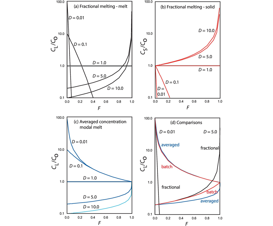
The enrichment of a trace element in a melt relative to its source (CL/Co) as a function of the fraction of melting (F), during modal fractional melting for different values of bulk partition coefficient (D). During fractional melting only a very small melt fraction is produced and it is instantly removed from the source. (a) Relative concentrations in the melt fraction during modal fractional melting. (b) Relative concentrations in the unmelted solid residue during modal fractional melting. (c) Relative concentrations in the melt fraction during modal fractional melting. In this case small melt fractions are removed instantly from the source but aggregate together and the composition averaged. This process produces very similar results to that of batch melting. (d) A comparison between the effects of batch melting (red curves), fractional melting (black curves), and averaged fractional melting (blue curves) for incompatible elements (D = 0.01) and compatible elements (D = 5).
When several melt increments have collected together the general expression becomes
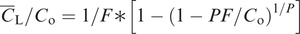
where 
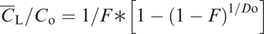
The relative enrichment of trace elements in the melt relative to the source during fractional melting in which the melt increments are collected together in a common reservoir is illustrated in Figure 4.10c. In this case fractional melting is indistinguishable from batch melting except for compatible elements at very large degrees of melting (Figure 4.9a).
A comparison between the degrees of relative enrichment during batch melting, fractional melting, and averaged fractional melting is shown in Figure 4.10d for highly incompatible elements (D = 0.01) and compatible elements (D = 5). For incompatible elements there is a large difference in concentration ratios between fractional melting and batch melting. Ratios for averaged fractional melting are very close to those for batch melting. For compatible elements there is little difference between the three models until high melt fractions of >20% are reached.
(c) Dynamic melting. Batch melting and fractional melting might be regarded as end-members of two different modes of melt extraction. However, studies of mid-ocean ridge basalts in the 1970s and 1980s suggested that mantle melting was a more complex and dynamic process than is implied by either batch or fractional melting (Langmuir et al., 1978; Wood, 1979; McKenzie, 1985). These processes have been reviewed by Shaw (2006) and discussed in detail by Shaw (2000) and Zhou and Reid (2001). These authors propose numerical models for dynamic melting, by which they mean continuous melting with retained or trapped melt. This process may take place in either a closed or open system. In a closed system a melt may leave the system but nothing is added, whereas in an open system matter is being added while solid material melts and melt is being released. During dynamic melting trace element concentrations in the melt will be influenced by variable melt/source-rock ratios, a variable contribution of solid phases to the melt (modal or non-modal melting), as well as varying partition coefficients. In part the process is also governed by the permeability threshold, that is, the critical degree of melting at which melt first leaves the system. The effects of dynamic melting and the importance of the interstitial melt fraction on the relative concentrations of an incompatible element during non-modal melting of mantle peridotite are illustrated as a function of total melt fraction in Figure 4.11. The limiting concentrations are given by the batch melting and fractional melting curves and the continuous melting curves have a shape similar to that of the fractional melting curves. However, the models discussed by Shaw (2000) are limited inasmuch as they do not account for variable partition coefficients; melting proportions are held constant; and kinetic diffusion effects are ignored.
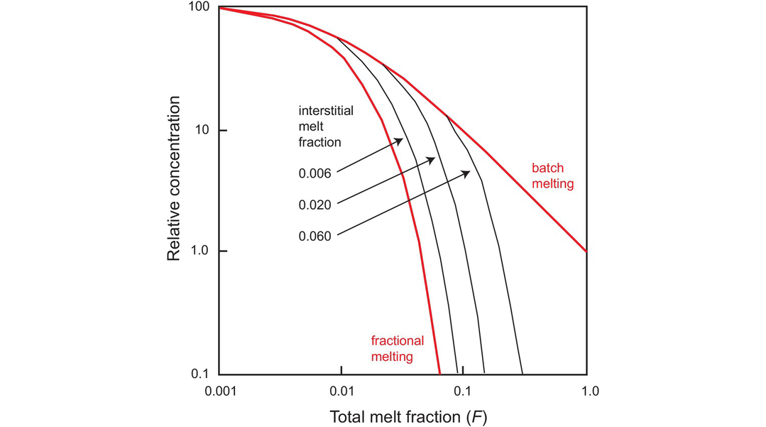
Behaviour of an incompatible element during the non-modal melting of peridotite. The limiting cases are batch melting and fractional melting. Dynamic melting defines relative concentration curves similar to that of fractional melting but shows a dependence on the value of the interstitial melt fraction. Three such curves are shown.
(d) Zone refining. Zone refining or zone melting is a process used in metallurgy for the purification of metals. The principle is that a metal rod or some similar material is passed through a heat source which causes melting of a small section of the rod. During this melting, incompatible impurities in the metal accumulate in the melt. As the rod is passed through the heat source the melt migrates and scavenges impurities as it moves. The end products are a metal rod depleted in impurities and a final melt enriched in impurities.
The equation for the enrichment of a trace element in the melt (CL) relative to the original composition (Co) by zone refining is
The depletion in the source (CS) relative to the concentration in the original composition is
where n is the number of equivalent rock-volumes that have reacted with the liquid. Where n is very large the CL/Co reduces to 1/D. The numerical effects of zone refining are illustrated in Figure 4.12, which shows the enrichment of a trace element relative to its original concentration for the number of rock volumes consumed (n). For incompatible elements (0.001–0.01) the maximum enrichment in the melt is 1/D rock volumes. In the solid phase CS/Co rises to 1.0 after a large number of rock volumes (see also Shaw, 2006).
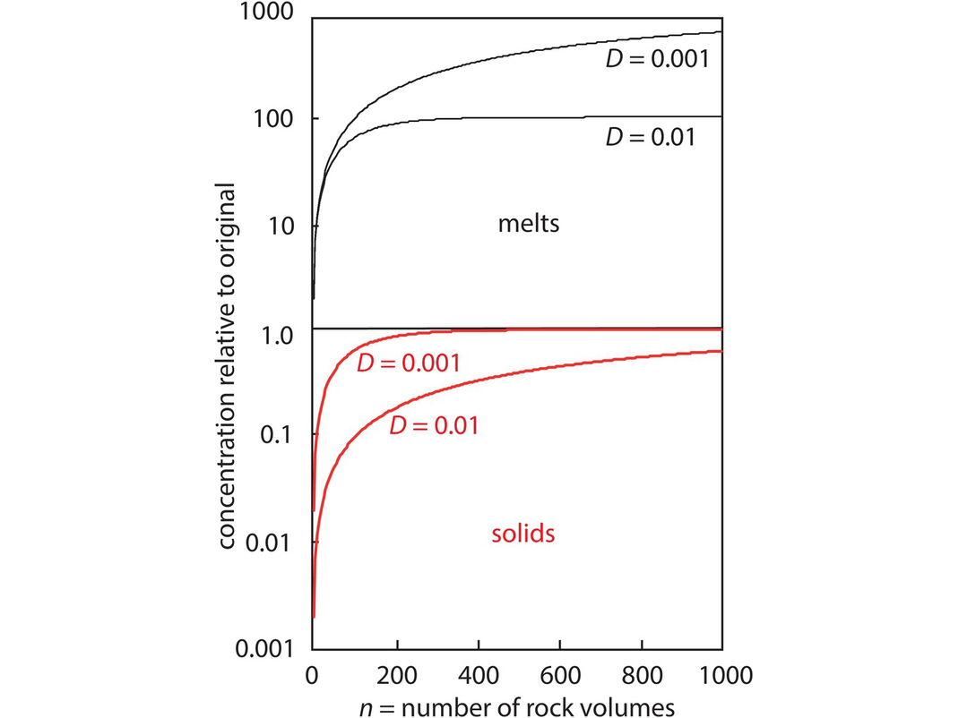
Plot of trace element enrichment during zone refining in both the melt and residual solid for incompatible elements with D = 0.01 and 0.001. The solid phase approaches the original composition and the melt phase the value of 1/D (the partition coefficient) after a large number of rock volumes.
Originally, zone refining was thought to be applicable to mantle processes (Harris, 1974) and Neal and Davidson (1989) proposed a zone-refining process to model REE concentrations in a highly enriched potassic ultramafic rock parental to alnöite at Malaita in the Solomon Islands. However, it is now thought that most highly enriched mantle melts are the product of fractional melting in a dynamic melting environment (see above). Thus, most recent applications of zone refining involve the presence of a fluid phase and have been applied to the development of fluid inclusions (Lambrecht and Diamond, 2014), mineralisation in layered mafic intrusions (Brűgmann et al., 1989), the development of chimneys in hydrothermal vent systems (Yuan et al., 2018) and in the formation of granitoid magmas (Lundstrom, 2009).
4.2.2.3 Crystal Fractionation
This section examines the way in which trace elements behave during the crystallisation of a silicate melt and applies principally to magma chamber processes. Five types of crystallisation are considered: equilibrium crystallisation, Rayleigh fractionation, in situ crystallisation, assimilation and fractional crystallisation (AFC), and dynamic processes in a replenished magma chamber.
(a) Equilibrium crystallisation. The starting point of equilibrium crystallisation is a closed system in which a hot magma cools until one or more mineral phases begins to crystallise. The process describes complete equilibrium between all solid phases and the melt during crystallisation. This is not thought to be a common process, although the presence of unzoned crystals in some mafic rocks suggests that it may be applicable on a local scale in some mafic magmas. The distribution of trace elements during equilibrium crystallisation is the reverse of equilibrium or batch melting (Section 4.2.2), and the equation therefore is
The equation for the crystallising solids is
In this case Co is redefined as the initial concentration of a trace element in the initial melt, CR the concentration of a trace element in the crystallising solid, F is the fraction of melt remaining and D is the bulk partition coefficient of the fractionating assemblage. The enrichment and depletion of trace elements relative to the original liquid for a range of partition coefficients is identical to that in the batch melting diagram (Figure 4.9a), but in this case the value of F (the fraction of melt remaining) is shown decreasing from left to right on the diagram (see Figure 4.13a).
(b) Fractional crystallisation/Rayleigh fractionation. More commonly, crystals are thought to be removed from the site of formation after crystallisation and the distribution of trace elements is not an equilibrium process. At best, surface equilibrium may be attained, and so fractional crystallisation is better described by the Rayleigh law. Rayleigh fractionation describes the extreme case where crystals are effectively removed from the melt the instant they have formed. The equation for Rayleigh fractionation is
and the equation for the enrichment of a trace element relative to the original liquid in the crystals as they crystallise (the instantaneous solid) CR is given by
The equation for the mean enrichment of a trace element in the cumulate relative to the original liquid – the total residual solid 
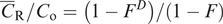
Rayleigh fractionation is illustrated in Figure 4.13a and shows the concentration of a trace element relative to its initial concentration in the liquid at differing values of F – the proportion of liquid remaining – for different values of D. For incompatible elements there is little difference between Rayleigh fractionation and equilibrium crystallisation until more than about 75% of the magma has crystallised at which point the efficient separation of crystals and liquid becomes physically difficult. The limiting case for incompatible elements is where D = 0 in which case CL/CO = 1/F, the same as for equilibrium crystallisation. It is therefore impossible to enrich a liquid beyond this point by fractional crystallisation. Rayleigh fractionation is less effective than batch melting in changing the ratio of two incompatible elements for the Rayleigh fractionation curve, for D = 0.01 plots very close to the curve for D = 0.1. Compatible elements are removed from the melt more rapidly than in the case of equilibrium crystallisation (Figure 4.13a).
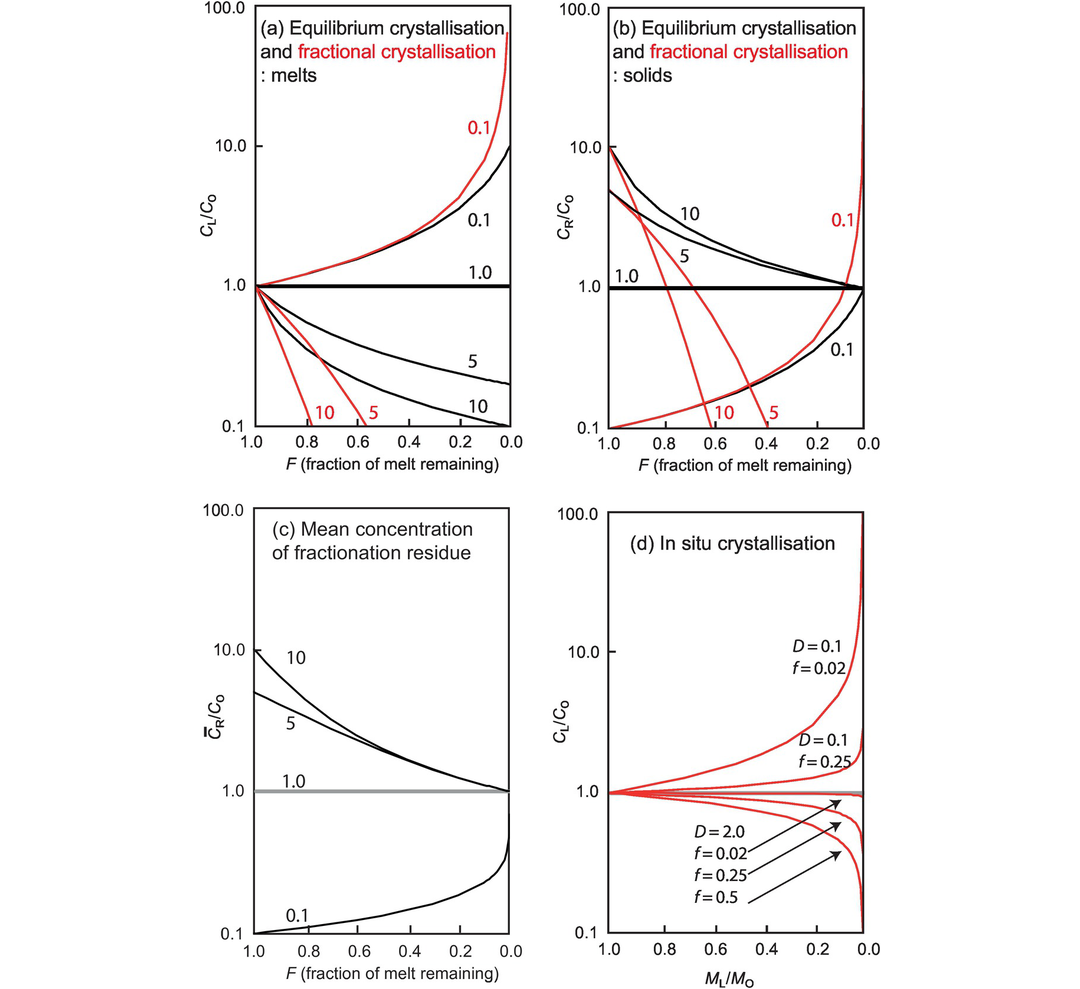
Relative concentrations versus fraction of melt remaining for trace elements in different crystallisation models for a range of partition coefficients (values shown adjacent to respective curves). (a) Relative concentrations in the melt during equilibrium crystallisation (black lines) and fractional crystallisation (red lines) for partition coefficient with values between 0.1 and 10; (b) relative concentrations in the solid residue during equilibrium crystallisation (black lines) and fractional crystallisation (red lines) for partition coefficient with values between 0.1 and 10; (c) average relative concentration in the accumulated solid residue during fractional crystallisation for partition coefficient with values between 0.1 and 10; (d) concentration in the melt during in situ crystallisation for D = 0.1 and f = 0.02 and 0.25 (f is the fraction of magma allocated to the solidification zone which is returned to the magma chamber) and for D = 2.0 and f = 0.02 and 0.5.
The concentration of trace elements in the instantaneous solid residue of Rayleigh fractionation is illustrated in Figure 4.13b. More relevant, however, is the mean concentration in the cumulate (
(c) In situ crystallisation. It is also important to consider a more realistic view of fractional crystallisation in a magma chamber in which there is not a perfect separation of crystals and melt. Langmuir (1989) proposed that fractional crystallisation is an in situ process in which residual liquid is separated from a crystal mush – rather than vice versa – and that this takes place in a solidification zone at the magma chamber margin. The solidification zone is located between the cumulate pile and the magma, and it progressively moves through the magma chamber until crystallisation is complete. The equation which describes trace element concentrations in the melt during in situ crystallisation is presented for the simplified case where there is no trapped liquid in the solidification zone (Langmuir, 1989). This allows us to compare the results with the effects of fractional and equilibrium crystallisation. The relevant equation is
where Mo is the initial mass of the magma chamber and ML is the mass of liquid remaining so that the ratio (ML/Mo) is equivalent to the term (F) – the fraction of melt remaining in equilibrium and fractional crystallisation models. The variable f is the fraction of magma allocated to the solidification zone which is returned to the magma chamber. Eq. 4.23 is similar in form to the Rayleigh fractionation equation but with a more complex exponent. The effects of in situ crystallisation on the ratio of a trace element relative to the parental magma (CL/Co) for different melt fractions returned to the magma chamber (f = 0.02–0.5) is shown for two different bulk partition coefficients in Figure 4.13d. The chief differences between in situ crystallisation and Rayleigh fractionation may be observed by comparing Figures 4.13a and d. The limiting case is where f = 1.0 which is Rayleigh fractionation. At low values of f, the enrichment of incompatible elements and the depletion of compatible elements are not as extreme during in situ fractional crystallisation as in Rayleigh fractionation.
Alternative approaches to modelling incomplete fractional crystallisation include the influence of a trapped melt. A range of models is summarised by Shaw (2006). For a simple model in which the composition of the trapped melt is identical to that in the magma chamber, then the relative enrichment of a trace element is given by
where F is the degree of fractionation, x is the proportion of trapped melt, and D is the bulk partition coefficient. In general, the effect of in situ crystallisation on trace element concentrations, whether in a solidification zone or as the effects of a trapped melt, is to reduce the degree of fractionation.
(d) Assimilation and fractional crystallisation. It was Bowen (1928) who first proposed that the latent heat of crystallisation generated during fractional crystallisation may lead to wall-rock assimilation in the magma chamber (see Section 3.3.1). In practical terms this may be evidenced by the presence of xenoliths of country rock within magmatic rocks. Petrologically, the process of crustal assimilation is likely to be important in understanding the geochemistry of magmas erupted through the continental crust, for in this tectonic setting it is necessary to remove the effects of country rock assimilation before the composition of primary magmas can be established.
The first quantitative model in which assimilation and fractional crystallisation (AFC) were seen as coupled processes was given by DePaolo (1981b), who described the concentration of trace elements, and stable and radiogenic isotope ratios, in a melt relative to the composition of the original magma. The general equation is given by DePaolo (1981b) and is
where r is the ratio of the assimilation rate to the fractional crystallisation rate and is kept constant, D is the bulk partition coefficient (also kept constant), CL is the element concentration in the contaminated magma, CA is the concentration of the trace element in the assimilated wall rock and f′ is described by the relationship f′ = F −(r−1+D)/(r−1) in which F is the fraction of magma remaining and D is the bulk distribution coefficient.
In subsequent studies Powell (1984) inverted the DePaolo (1981b) equations in order to characterise the chemistry of contaminants involved in magma evolution from observed isotope and trace element relationships, and Aitcheson and Forrest (1994) provided a graphical solution to calculate the proportion of crust assimilated relative to the mass of the magma. Cavazzini (1996) added the caveat that the time-averaged mass of assimilated crust can be significantly different from the instantaneous mass of material assimilated. More recently, Guzman et al. (2014) developed software to provide solutions to the equations of DePaolo (1981b) and Aitcheson and Forrest (1994). Other relevant studies include Cribb and Barton (1996), who extended the DePaolo (1981b) model to include the case where r is not constant and the mass of assimilated crust is decoupled from the mass crystallised, and Nishimura (2012, 2013), who provided a model and associated software for AFC processes which accommodate the effects of the imperfect separation of crystals from the melt. More advanced modelling based on the energy-constrained AFC (EC-AFC) models of Bohrson and Spera (2001, 2007) and Spera and Bohrson (2001), and the Magma Chamber Simulator of Bohrson et al. (2014), are used to model crystallization, magma recharge and assimilation processes by coupling thermodynamically based phase equilibria solutions to constraints based on trace elements and isotope geochemistry (Heinonen et al., 2019).
During AFC processes the concentration of a trace element in the final melt relative to the concentration in the initial parental magma is dependent on the fraction of melt remaining and the bulk distribution coefficient. This is illustrated in Figure 4.14 which shows two ratios for the rate of assimilation (r = 0.2 and 0.8), different ratios for the concentration of the trace element in the assimilant relative to the parent magma (CA/Co) = 0.1, 10 and 100) for different values of D (0.1 and 2). Where the rate of assimilation to fractional crystallization is small (r = 0.2) and the ratio of the concentration of the trace element in the assimilant relative to the parental magma (CA/Co) is small, incompatible elements behave in a manner similar to Rayleigh fractionation. However, as the value of (CA/Co) increases the concentration in the final melt rises rapidly even when there is a large fraction of melt remaining. Depletion in compatible elements is less dramatic than in Rayleigh fractionation for low CA/Co values, and when the relative concentration of the trace element in the assimilant is higher than that in the primary magma, the final melt is enriched relative to the initial melt. For very compatible elements concentrations level off after a small degree of fractionation. Where the rate of assimilation is high (r = 0.8) and the concentration of the trace element in the assimilant relative to the parental magma (CA/Co) is small, incompatible elements are enriched and there is some separation between incompatible and strongly incompatible elements (Figure 4.14b). In contrast, compatible elements are strongly depleted. As the trace element concentration in the assimilant increases relative to the parental melt (CA/Co), compatible elements are enriched (Figure 4.14b).
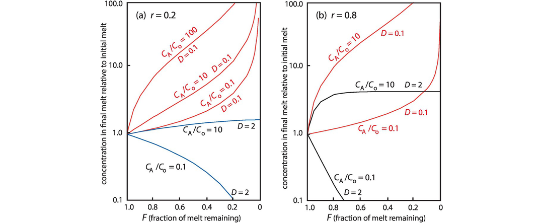
The concentration of trace elements in the final melt composition relative to the initial melt composition during AFC processes. The relative concentrations for incompatible element (D = 0.1) and a compatible element (D = 2) are plotted against the fraction of melt remaining in the magma chamber (F) during assimilation and fractional crystallisation for two different values of r (the ratio of the assimilation rate to the fractional crystallisation rate) and at a range of concentrations in the assimilant relative to the parental magma (CA/Co) (Eq. 4.25).
AFC processes can be difficult to recognise on the basis of geochemistry alone for they require a strong contrast in trace element concentrations between magma and wall rock before they can be detected (Powell, 1984). For this reason, where field observations are available they should be included in formulating any hypothesis of AFC processes. The large number of variables in Eq. 4.25 means that the results plotted in Figure 4.14 will not provide a unique solution to the relative proportion of crustal assimilated into the magma. For this purpose, readers should follow the methods of Aitcheson and Forrest (1994) and Guzman et al. (2014).
(e) Dynamic fractionation: the RTF magma chamber. In an attempt to view magma chamber processes in a dynamic way, O’Hara (1977) and O’Hara and Matthews (1981) proposed a model to describe the behaviour of trace elements in a periodically replenished, periodically tapped, continuously fractionated magma chamber (abbreviated to RTF). In other words, this is an open magmatic system. Support for this approach comes from the petrology and geochemistry of layered mafic igneous intrusions and their associated lavas such as those from the Isle of Skye in Scotland (Fowler et al., 2004).
O’Hara (1977) and O’Hara and Matthews (1981) proposed that the life of a magma chamber comprises a series of cycles, each of which has four stages: fractional crystallisation, magma eruption, wall-rock contamination and replenishment. The simplest form of this model is where all parameters (melt fractions and partition coefficients) remain constant during the life of the magma chamber, there is no assimilation, the mass fractions of melt escaping and that being added to the system are small, and the melt is in a steady state. That is, the volume of melt leaving the system through crystallisation and eruption is the same as the volume melt added to system, so that the magma chamber maintains a constant volume of melt. In this case the concentration of a trace element in the steady state melt produced after a large number of cycles (ssCB) relative to the concentration in the parent magma (Co) is given by the expression
where x is the mass fraction of the liquid lost to crystallisation in each cycle, y is the mass fraction of the liquid escaping in each cycle, and D is the bulk distribution coefficient.
O’Hara and Matthews (1981) also provide a more general, iterating equation for the RTF magma chamber for the concentration of an element in a mixed magma after multiple cycles (see their Eq. 9). In the special case where x + y = 1, that is, the magma chamber is emptied, then
which is the Rayleigh fractionation equation.
If x and y are very small, then
When D = 0, that is, in the case of a totally incompatible trace element,
and is a measure of the maximum enrichment attainable.
The degree of enrichment in the melt ssCB /Co (calculated using Eq. 4.26) is plotted against x, the mass fraction of liquid crystallised in each cycle (Figure 4.15). Assuming y = 0.1, the mass of melt crystallised for several different values of D shows that during dynamic fractionation the relative concentrations of compatible elements are similar to those produced during Rayleigh fractionation, but for the incompatible elements small changes in partition coefficient show measurable concentration differences at moderate x-values.
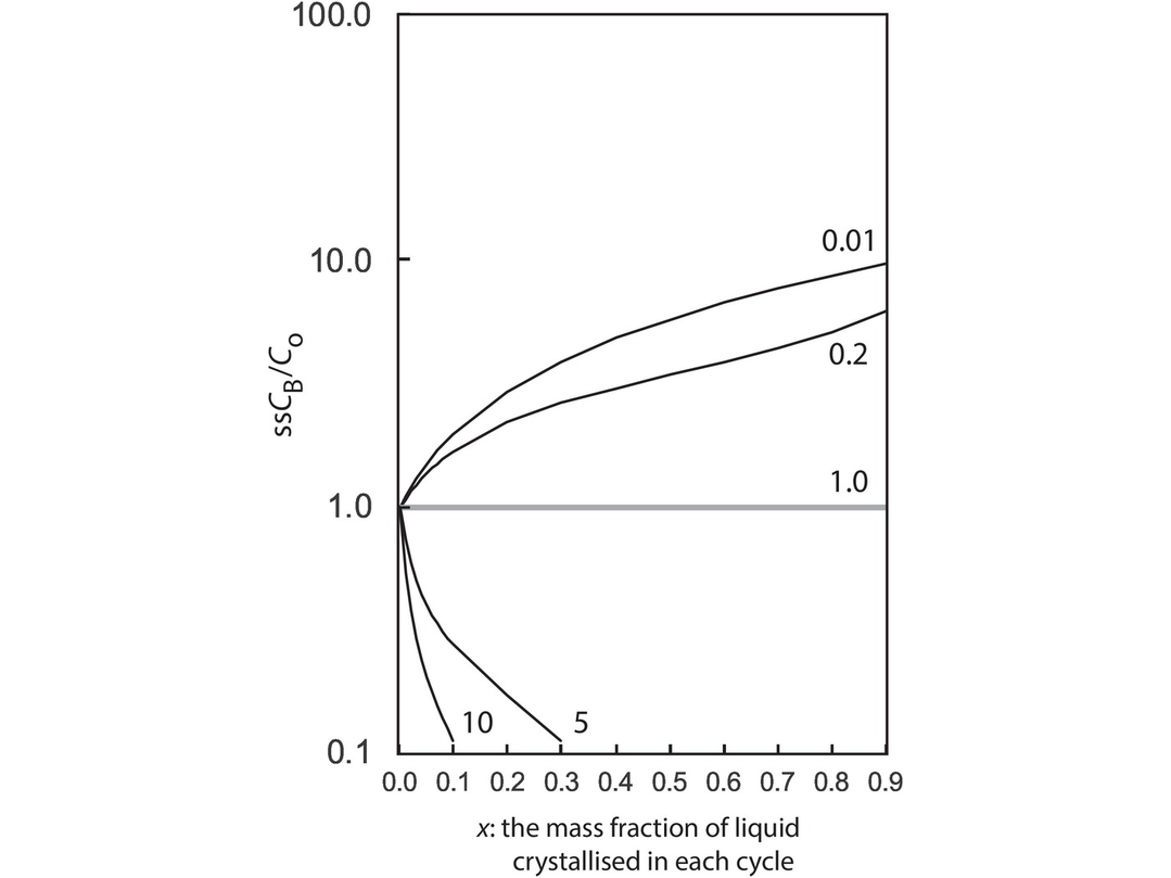
The degree of enrichment ssCB /Co versus x (the mass fraction of liquid crystallised in each RTF cycle) for a range of partition coefficients. y (the mass fraction of the liquid lost to crystallisation in each cycle) = 0.1. Note the difference in relative concentration between the incompatible and moderately incompatible element for low and intermediate values of x.
Since the early work of O’Hara (1977) and O’Hara and Matthews (1981) there have been a number of subsequent studies, which are summarised in Shaw (2006), Bohrson et al. (2014) and Nishimura (2019), and the consensus is that despite the dynamic nature of the processes involved in RTF magma chambers, trace element concentrations appear to show steady state behaviour. A particular and perhaps diagnostic feature of RFT processes is that ‘significant changes can occur in the ratio of highly incompatible and moderately incompatible elements (D = 0.01–0.2)’ (O’Hara and Matthews, 1981), although Langmuir (1989) points out that these properties are also very similar to those characterising in situ crystallisation processes discussed above and that care needs to be taken to discriminate between the two processes.
4.2.2.4 Sedimentary Processes
Trace element concentrations in sediment result from the competing influences of the provenance, weathering, diagenesis, sediment sorting and the aqueous geochemistry of the individual elements. For the most part, however, these processes have not been quantified in the same way as in igneous rocks. A notable exception is the field of low-temperature aqueous geochemistry in which advanced quantitative models developed by Bethke (2012) have been applied to chemical models of river water and seawater, to the formation of hydrothermal mineral deposits and to understanding the processes of weathering, sediment diagenesis and acid drainage.
Most trace elements have very low concentrations in river and seawater, and controls on their REE concentrations are discussed in Section 4.3.3.2. In sediments the highest concentrations of trace elements are found in clay-rich sediments, and most geochemical studies have concentrated on these. There is an extensive literature on the trace element geochemistry of shales. In particular, selected trace elements may be used to identify specific geochemical processes but also are important in identifying the provenance of sediments. The most important elements in this respect are the REE, Th, Sc and to a lesser extent Cr and Co. These elements have very low concentrations in seawater and river waters, low residence times in the ocean, and element ratios which are unaffected by diagenesis and metamorphism. Thus, they represent the terrigenous component of sediment and reflect the chemistry of their source (see Sections 4.3.3.3 and 4.6.2). Other immobile elements such as Zr, Hf and Sn may be mechanically distributed according to grain size and be controlled by the concentration of the so-called accessory heavy minerals.
The more soluble trace elements include Fe, Mn, Pb and sometimes Cr, and these can be mobile during diagenesis. During weathering the elements Cs, Rb and Ba are fixed but Sr can be leached. In chemical sediments trace element concentrations are most likely to reflect the composition of the water from which they were precipitated: seawater, pore water, or hydrothermal fluids (see Section 4.3.3.3).
4.3 The Rare Earth Elements (REE)
The rare earth elements (REE) are amongst the most useful of all trace elements in evaluating a wide range of processes in igneous, sedimentary and metamorphic petrology, and also make an important contribution to cosmochemistry. In geochemistry the REE, more accurately known as the lanthanide REE, comprise the series of metals with atomic numbers 57–71 (the elements La to Lu, Table 4.6). In addition, the element Y has an ionic radius similar to that of the REE and is sometimes included with them. Typically, elements with low atomic numbers in the series are termed the light rare earth elements (LREE), those with the higher atomic numbers the heavy rare earth elements (HREE), and less commonly the middle members of the group (Sm to Ho) are known as the middle rare earth elements (MREE).
| Atomic number | Name | Symbol | Ionic radius for eight-fold coordinationa | |
|---|---|---|---|---|
| 57 | Lanthanum | La | La3+ | 1.160 |
| 58 | Cerium | Ce | Ce3+ | 1.143 |
| Ce4+ | 0.970 | |||
| 59 | Praesodymium | Pr | Pr3+ | 1.126 |
| 60 | Neodymium | Nd | Nd3+ | 1.109 |
| 61 | Promethium | Pm | not naturally occurring | |
| 62 | Samarium | Sm | Sm3+ | 1.079 |
| 63 | Europium | Eu | Eu3+ | 1.066 |
| Eu2+ | 1.250 | |||
| 64 | Gadolinium | Gd | Gd3+ | 1.053 |
| 65 | Terbium | Tb | Tb3+ | 1.040 |
| 66 | Dysprosium | Dy | Dy3+ | 1.027 |
| 67 | Holmium | Ho | Ho3+ | 1.015 |
| 68 | Erbium | Er | Er3+ | 1.004 |
| 69 | Thulium | Tm | Tm3+ | 0.994 |
| 70 | Ytterbium | Yb | Yb3+ | 0.985 |
| 71 | Lutetium | Lu | Lu3+ | 0.977 |
| 39 | Yttrium | Y | Y3+ | 1.019 |
4.3.1 The Chemistry of the REE
The REE all have very similar chemical and physical properties. This arises from the fact that they all form stable 3+ ions of similar size. Typically, they substitute for large major element cations such as Ca2+ which has a similar ionic radius of 1.12 Å in eight-fold coordination. Such differences as there are in chemical behaviour are a consequence of the small but systematic decrease in ionic size with increasing atomic number, known in chemistry as the lanthanide contraction. This is illustrated for ions in eight-fold coordination state in Table 4.6. These small differences in size and behaviour are exploited by a number of petrological processes causing the REE series to become fractionated relative to each other. It is this phenomenon which is used in geochemistry to probe into the genesis of rock suites and unravel petrological processes. A small number of the REE also exist in oxidation states other than 3+ but the only ions of geological importance are Ce4+ and Eu2+. These form a smaller and a larger ion, respectively, relative to the 3+ oxidation state and may be a useful monitor of redox conditions. A detailed review of the geochemistry of the REE is given by McLennan and Taylor (2012) and discussion of REE mineralisation and its importance in modern technology by Chakhmouradian and Wall (2012).
4.3.2 Presenting REE Data
Rare earth element concentrations in rocks are usually normalised to a reference standard or particular rock type (Section 4.3.2.5). Chondritic meteorites are a common reference standard chosen because they are thought to be the most primitive, least fractionated samples of the solar system dating from the time of nucleosynthesis. However, the concentrations of the REE in the solar system are highly variable because of the different stabilities of the atomic nuclei. REE with even atomic numbers are more stable, and therefore more abundant, than REE with odd atomic numbers, thus producing a zig-zag pattern on a composition–abundance diagram (Figure 4.16a) known as the Oddo–Harkins effect. This pattern of abundance is also found in natural samples, and so chondritic normalisation has two important functions. First, it eliminates the abundance variation between odd and even atomic number elements, producing a smooth curve, and, second, it allows any fractionation of the REE group relative to chondritic meteorites to be easily identified. Normalised values and ratios of normalised values are denoted with the subscript N – hence, CeN, (La/Ce)N, and so on. The REE are normally presented on a normalised concentration versus atomic number diagram, although O’Neill (2016) has recommended using the 3+ ionic radius as the x-axis rather than the atomic number. The advantage of using ionic radii is that the resulting pattern is generally smoother and highlights any anomalies; it is also amenable to the fitting of a polynomial which may be used in petrogenetic interpretation (O’Neill, 2016). Concentrations are plotted on the y-axis, normalised to the chondritic reference value, and expressed as the logarithm to the base 10 of the value. Concentrations at individual points on the graph are joined by straight lines (Figure 4.16b). It is normal to plot the full range of atomic numbers (57–71) on the x-axis, even if not all the REE have been measured (e.g., Pm). This type of REE diagram is sometimes referred to as the Masuda–Coryell diagram after the original proponents of the diagram (Masuda, 1962; Coryell et al., 1963). Trends on REE diagrams are usually referred to as REE patterns and the shape of a REE pattern is of considerable petrological interest.
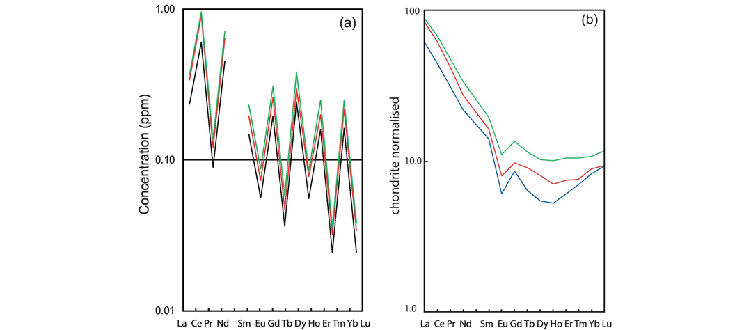
Plots of REE concentration. (a) REE concentrations in ppm for selected CI chondrites plotted against atomic number. REE with even atomic numbers have higher concentrations than those with odd atomic numbers. These values are used to normalise rock REE concentrations. The green line represents the data of Taylor and McLennan (1985) (column 12 in Table 4.7), the red line the data of Wakita et al. (1971) (column 9 in Table 4.7), and the black line the data of Anders and Grevesse (1989) (column 3 in Table 4.7). (b) An example of a chondrite normalised plot showing the REE plotted by atomic number on the x-axis and CI chondrite normalised concentrations plotted on a log scale y-axis. The data are for plagiogranites from the mantle section of the Oman ophiolite and are samples 13–18, 13–19 and 13–21 from Rollinson (2015). They are normalised using the values of Barrat et al. (2012) (Table 4.7, column 7). The samples show negative Eu anomalies with Eu/Eu* = 0.55–0.68.
The plotted position of Eu may lie off the general trend defined by the other elements on a REE diagram (Figure 4.16b) and this defines a europium anomaly. If the plotted composition lies above the general trend, then the anomaly is described as positive; and if it lies below the trend, then the anomaly is said to be negative. Europium anomalies may be quantified by comparing the measured concentration (Eu) with an expected concentration obtained by interpolating between the normalised values of Sm and Gd to calculate Eu*. Thus the ratio Eu/Eu* is a measure of the europium anomaly; a value of greater than 1.0 indicates a positive anomaly, and a value of less than 1.0 is a negative anomaly.
Taylor and McLennan (1985) recommend using the geometric mean to calculate the Eu anomaly:
In a similar manner, Ce anomalies can be quantified:
Normally anomalies should be less than 0.95 or greater than 1.05 to be considered significant.
4.3.2.1 Difficulties with Chondrite Normalisation
There are a large number of different values determined for the composition of chondritic meteorites, and so it is important to explore how this range of values has arisen and the implications this has for appropriate normalisation values. The logic behind chondrite normalisation is that chondrites represent the undifferentiated material of the solar system, and so any divergence from these values is indicative of a process or set of processes that has operated on the Earth. It is important therefore to identify the most primitive of the chondrites as the reference point for the least differentiated materials of the solar system. Older chondrite analyses of the REE were based upon data for ordinary chondrites (Haskin et al., 1968), whereas CI (letters ‘C’ and ‘I’) carbonaceous chondrites do not contain chondrules (early solar system melts) and represent the least thermally altered samples of the early solar system. However, there are some difficulties with this approach:
CI chondrites are extremely rare. There only five known and the largest is the Orgueil meteorite, a 14-kg meteorite which fell in France in 1868.
Measurements are normally made using very small quantities of meteorite material. It is unclear how heterogeneous chondritic meteorites are (Barrat et al., 2012).
Carbonaceous chondrites are rich in volatiles. Comparative studies must take account of possible differences in volatile content.
Difference analytical approaches have been used to measure REE in chondrites. Early studies used neutron activation (INAA), although this method can analyse only for a subset of the REE, whereas more recent measurements are made by isotope dilution (IDMS) and ICP-MS.
4.3.2.2 Choosing a Set of Normalising Values
There are currently two different approaches to selecting an appropriate set of chondritic reference values for normalising the REE. Some authors normalise to the average composition of ordinary chondrites, whereas others use an average of CI chondrites. The ordinary chondrite values are higher than the CI chondrite values. Some typical normalising values currently in use are given in Table 4.7.
| Averaged CI chondrite | ‘Older’ ordinary chondrite | CI chondrite (recalculated volatile free) | ||||||||||||||
|---|---|---|---|---|---|---|---|---|---|---|---|---|---|---|---|---|
| 1 | 2 | 3 | 4 | 5 | 6 | 7 | 8 | 9 | 10 | 11 | 12 | 13 | 14 | |||
| La | 0.2370 | 0.2370 | 0.2347 | 0.2360 | 0.2420 | 0.2469 | 0.2350 | 0.24460 | 0.340 | 0.330 | 0.3670 | 0.3670 | 0.3191 | 0.3100 | ||
| Ce | 0.6120 | 0.6130 | 0.6032 | 0.6190 | 0.6220 | 0.6321 | 0.6000 | 0.63790 | 0.910 | 0.880 | 0.9570 | 0.9570 | 0.8201 | 0.8080 | ||
| Pr | 0.0950 | 0.0928 | 0.0891 | 0.0900 | 0.0946 | 0.0959 | 0.0910 | 0.09637 | 0.121 | 0.112 | 0.1370 | 0.1370 | 0.1211 | 0.1220 | ||
| Nd | 0.4670 | 0.4570 | 0.4524 | 0.4630 | 0.4710 | 0.4864 | 0.4640 | 0.47380 | 0.640 | 0.600 | 0.7110 | 0.7110 | 0.6151 | 0.6000 | ||
| Sm | 0.1530 | 0.1480 | 0.1471 | 0.1440 | 0.1520 | 0.1556 | 0.1530 | 0.15400 | 0.195 | 0.181 | 0.2310 | 0.2310 | 0.2000 | 0.1950 | ||
| Eu | 0.0580 | 0.0563 | 0.0560 | 0.0547 | 0.0578 | 0.0599 | 0.0586 | 0.05802 | 0.073 | 0.069 | 0.0870 | 0.0870 | 0.0761 | 0.0735 | ||
| Gd | 0.2055 | 0.1990 | 0.1966 | 0.1990 | 0.2050 | 0.2003 | 0.2060 | 0.20430 | 0.260 | 0.249 | 0.3060 | 0.3060 | 0.2673 | 0.2590 | ||
| Tb | 0.0374 | 0.0361 | 0.0363 | 0.0353 | 0.0384 | 0.0378 | 0.0375 | 0.03745 | 0.047 | 0.047 | 0.0580 | 0.0580 | 0.0494 | 0.0474 | ||
| Dy | 0.2540 | 0.2460 | 0.2427 | 0.2560 | 0.2550 | 0.2577 | 0.2540 | 0.25410 | 0.300 | nd | 0.3810 | 0.3810 | 0.3300 | 0.3220 | ||
| Ho | 0.0566 | 0.0546 | 0.0556 | 0.0552 | 0.0572 | 0.0554 | 0.0566 | 0.05670 | 0.078 | 0.070 | 0.0851 | 0.0851 | 0.0756 | 0.0718 | ||
| Er | 0.1655 | 0.1600 | 0.1589 | 0.1620 | 0.1630 | 0.1667 | 0.1660 | 0.16600 | 0.200 | 0.200 | 0.2490 | 0.2490 | 0.2160 | 0.2100 | ||
| Tm | 0.0255 | 0.0247 | 0.0242 | 0.0220 | 0.0261 | 0.0261 | 0.0262 | 0.02561 | 0.032 | 0.030 | 0.0356 | 0.0356 | 0.0329 | 0.0324 | ||
| Yb | 0.1700 | 0.1610 | 0.1625 | 0.1660 | 0.1690 | 0.1694 | 0.1680 | 0.16510 | 0.220 | 0.200 | 0.2480 | 0.2480 | 0.2209 | 0.2090 | ||
| Lu | 0.0254 | 0.0246 | 0.0243 | 0.0245 | 0.0253 | 0.0256 | 0.0246 | 0.02539 | 0.034 | 0.034 | 0.0381 | 0.0381 | 0.0330 | 0.0322 | ||
| Y | 1.5700 | 1.5700 | 1.5600 | 1.5300 | 1.5300 | 1.3950 | 1.5600 | nd | nd | nd | 2.2500 | 2.1000 | 2.1210 | nd | ||
Notes: nd, no data.
References: 1, Sun and McDonough (1989); 2, McDonough and Sun (1995); 3, Anders and Grevesse (1989) average; 4, Anders and Grevesse (1989) Orgueil; 5, Lodders et al. (2009); 6, Pourmand et al. (2012); 7, Barrat et al. (2012); 8, Evensen et al. (1978); 9, Wakita et al. (1971); 10, Haskin et al. (1968); 11, Taylor and McLennan (2009); 12, Taylor and McLennan (1985); 13, Korotev (1996); 14, Boynton (1984).
(a) Normalisation to CI chondrites. A carefully evaluated data set is given by Anders and Grevesse (1989), who calculated a mean value for CI chondrites from all published data at the time and found good agreement between their average chondrite data and solar element abundances determined independently from spectroscopy. (This similarity strongly supports the view that CI carbonaceous chondrites are representative of primitive solar system materials). They report two sets of values: an average of all CI meteorite data and an average for the Orgueil meteorite (Anders and Grevesse, 1989). The values of Sun and McDonough (1989) and McDonough and Sun (1995) are almost identical and are also based on average values from previous studies.
More recent determinations include those of Lodders et al. (2009), who provided a new CI average based upon data for the Orgueil meteorite, and Pourmand et al. (2012), who provide a new average based upon new multi-collector ICP-MS measurements of eight CI chondrites (five Orgeuil, two Ivuna and one Alais). Barrat et al. (2012) made new analyses of the Orgueil meteorite and of two other CI meteorites (Ivuna and Alais) by ICP-sector field mass spectrometry. They present a new average analysis for the Orgueil meteorite and show that it compares well with that of previous workers, although they note that the value for Tm in Anders and Grevesse (1989) may be too low.
(b) Normalisation to ordinary chondrites (CI chondrite, calculated volatile-free). Normalisation to ordinary chondrites is a means of taking into account the volatile content of CI chondrites. These values typically use the better-determined CI concentrations and introduce a factor to make the concentrations similar in absolute magnitude to those found in ordinary chondrites. For example, Korotev (1996) uses the compilation of Anders and Grevesse (1989) for CI chondrites multiplied by a factor of 1.36. A similar approach was adopted by Taylor and McLennan (1985, 2009), who used the values of Evensen et al. (1978) multiplied by 1.5, and Boynton (1984), who also used the values of Evensen et al. (1978) multiplied by 1.267 in order to be consistent with the average values of Haskin et al. (1968) and Wakita et al. (1971).
The normalising values currently in use are given in Table 4.7. It can be seen that the CI chondrite values calculated volatile-free are as much as 50% larger than the averaged CI values. It is important, therefore, that authors cite the source of the normalising values that they choose to use. Figure 4.16a shows the normalising concentrations plotted on a log-concentration versus REE atomic number plot. This diagram shows the higher concentrations of REE with even atomic numbers (the Oddo–Harkins effect) and shows that the normalising values based upon CI chondrites are all very similar. An example of a typical REE plot is given in Figure 4.16b.
4.3.2.3 REE Ratio Diagrams
The degree of fractionation of a REE pattern can be expressed by the ratio of the normalised concentration of a light REE (La or Ce) divided by the normalised concentration of a heavy REE such as Yb or the trace element Y. Hence the ratio (La/Yb)N is often plotted against either CeN or YbN on a bivariate graph and is a measure of the degree of REE fractionation, that is, the steepness of the REE pattern, with changing REE content. This is particularly helpful for large REE data sets, for a single diagram can summarise the results of otherwise very crowded REE plots. Similar diagrams may be constructed to measure the degree of fractionation of subgroups within the REE. In this way the ratio (La/Sm)N might be indicative of the degree of light REE fractionation and a ratio such as (Gd/Yb)N indicative of heavy REE fractionation. These two variables might be combined in bivariate plots such as (La/Sm)N versus LaN or (Gd/Yb)N versus YbN to show the relative fractionation of the light or heavy REE, respectively. When a data set shows variable REE patterns, it can be helpful to screen them and group them on a (La/Sm)N versus (Gd/Yb)N diagram (Figure 4.17).
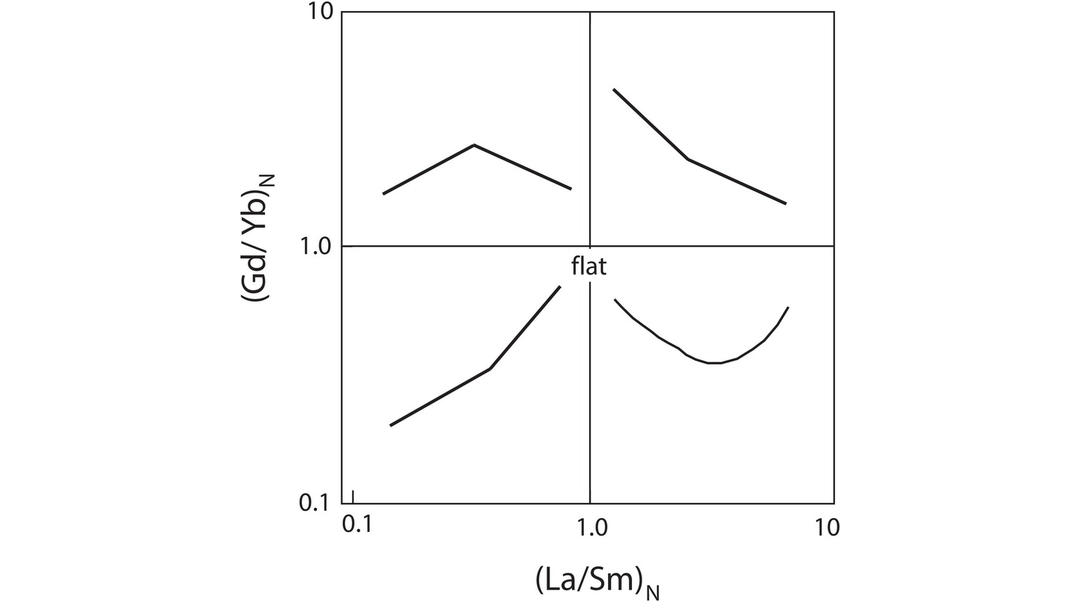
Log-log (La/Sm)N versus (Gd/Yb)N plot showing typical shapes of REE patterns indicated by the different quadrants of the diagram.
4.3.2.4 Shale Normalisation for Sediments
It has been observed that the concentration of many elements in fine-grained sedimentary rocks from continental platforms around the world is similar. This is a consequence of mixing through repeated cycles of erosion and the resultant ‘average sediment’ might be seen as an average composition of the Earth’s upper continental crust. Average shale compositions therefore are often used as the normalising value for REE concentrations in sedimentary rocks. Whether shale normalisation should be used rather than chondrite normalisation is governed by the nature of the problem to be solved. If the composition of a suite of sediments is to be compared to the average ‘background’ composition of the Earth’s upper crust – the likely source of the sediments – then shale normalisation is suitable. In this case any divergence from the shale value indicates the specific processes through which the sediment was produced. If chondrite normalisation is used, then the sediments are being compared with the primitive material of the solar system and divergence from the chondrite values will reflect the sum of all the processes that have taken place between the formation of the Earth and the formation of the sediment.
A range of commonly used shale averages is given in Table 4.8. Frequently, the reference sample chosen is continent-specific and includes the following:
In addition, a world shale average (WSA) has been proposed by Bau et al. (2018). The average value of the upper continental crust determined by Rudnick and Gao (2014) is based upon an average of surface derived samples, sediments and loess (Figure 4.18a). It has an identically shaped REE pattern to that of the shale samples, although the absolute REE concentrations in the average upper crust are slightly lower due to the dilution effect of REE-poor clastic and carbonate sediments. Relative to chondritic meteorites, shale averages have > 100 times light REE and show steep light REE patterns (La/Sm)N = 3.1–4.3. They have a small negative Eu anomaly and a relatively flat heavy REE pattern (Gd/Yb)N = 1.4–1.6, with about 20–30 times chondrite concentrations (Figure 4.18a).
| Sediment | Water | ||||||||||
|---|---|---|---|---|---|---|---|---|---|---|---|
| NASC ppm | MUQ ppm | PAAS ppm | ES ppm | WSA ppm | UCC ppm | Pacific 49-m depth ppm | Pacific 2576-m depth ppm | North Sea ppm | Rhine River ppm | MORT years | |
| 1 | 2 | 3 | 4 | 5 | 6 | 7 | 8 | 9 | 10 | 11 | |
| La | 32.00 | 32.51 | 44.56 | 44.300 | 40.30 | 31.00 | 1.25E-06 | 6.2E-06 | 2.89E-06 | 7.87E-05 | 1630 |
| Ce | 73.00 | 71.09 | 88.25 | 88.500 | 83.30 | 63.00 | 9.64E-07 | 2.17E-06 | 4.90E-06 | 2.90E-05 | 130 |
| Pr | 7.90 | 8.46 | 10.15 | 10.600 | 9.54 | 7.10 | 2.07E-07 | 9.44E-07 | 1.05E-06 | 5.35E-06 | 800 |
| Nd | 33.00 | 32.91 | 37.32 | 39.500 | 36.60 | 27.00 | 1.04E-06 | 4.38E-06 | 4.60E-06 | 2.31E-05 | 950 |
| Sm | 5.70 | 6.88 | 6.884 | 7.300 | 6.63 | 4.70 | 2.38E-07 | 8.78E-07 | 1.23E-06 | 1.27E-05 | 970 |
| Eu | 1.24 | 1.57 | 1.215 | 1.480 | 1.31 | 1.00 | 6.53E-08 | 2.34E-07 | 3.71E-07 | 1.46E-06 | 820 |
| Gd | 5.20 | 6.36 | 6.043 | 6.340 | 5.86 | 4.00 | 3.4E-07 | 1.33E-06 | 2.47E-06 | 1.10E-05 | 1100 |
| Tb | 0.85 | 0.99 | 0.8914 | 0.944 | 0.90 | 0.70 | 6.99E-08 | 2.13E-07 | 3.38E-07 | 9.98E-07 | 1130 |
| Dy | 5.80 | 5.89 | 5.325 | 5.860 | 5.66 | 3.90 | 4.49E-07 | 1.56E-06 | 2.40E-06 | 6.08E-06 | 1510 |
| Ho | 1.04 | 1.22 | 1.053 | 1.170 | 1.09 | 0.83 | 1.19E-07 | 4.26E-07 | 6.10E-07 | 1.32E-06 | 6800 |
| Er | 3.40 | 3.37 | 3.075 | 3.430 | 3.30 | 2.30 | 3.63E-07 | 1.44E-06 | 1.97E-06 | 3.92E-06 | 6800 |
| Tm | 0.50 | 0.51 | 0.451 | 0.492 | 0.48 | 0.30 | 5.07E-08 | 2.21E-07 | nd | nd | nd |
| Yb | 3.10 | 3.25 | 3.012 | 3.260 | 3.12 | 2.00 | 3.29E-07 | 1.51E-06 | 1.96E-06 | 3.78E-06 | nd |
| Lu | 0.48 | 0.49 | 0.4386 | 0.485 | 0.47 | 0.31 | 4.72E-08 | 2.68E-07 | 3.50E-07 | 6.57E-07 | nd |
| Y | 27.00 | 31.85 | 27.31 | 31.900 | 28.70 | 21.00 | 6.69E-06 | 2.24E-05 | 2.60E-05 | 3.75E-05 | 5100 |
Notes: nd, no data.
References: 1, North American shale composite (McLennan, 1989); 2, Queensland mud (Kamber et al., 2005); 3, post-Archaean average Australian sedimentary rock (Pourmand et al., 2012); 4, average European shale (Bau et al., 2018); 5, world shale average (Bau et al., 2018); 6, average upper continental crust (Rudnick and Gao, 2014); 7, northwest Pacific (49-m depth) (Alibo and Nozaki, 1999); 8, northwest Pacific (2576-m depth) (Alibo and Nozaki, 1999); 9, seawater, North Sea (Bau et al., 2018); 10, river water, Rhine (Bau et al., 2018); 11, mean oceanic residence time in years (Alibo and Nozaki, 1999).
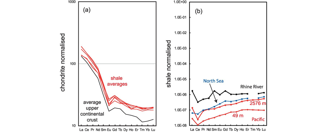
Sediment normalization. (a) Five average shale compositions (red) and the average composition of the upper continental crust (black) (from Table 4.8), plotted relative to their concentration in chondritic meteorites using the normalising values of Barrat et al. (2012). (b) The composition of ocean water and river water (Table 4.8) normalised to the composition of European shale (Table 4.8, column 4). The composition of filtered North Sea water and Rhine River water are from Bau et al. (2018) and the total dissolved concentrations of REE from two different depths in the northwest Pacific Ocean are from Alibo and Nozaki (1999). Note the different scales in (a) and (b).
4.3.2.5 Rock Normalisation
Some authors normalise REE concentrations to a particular sample in a rock suite as a measure of relative change. This is also useful when the REE concentrations of the individual minerals in the rock have also been determined, for then they can be expressed relative to the concentration in the whole rock as a means of showing where the REE are concentrated in the sample. A similar form of normalisation is used to express REE concentration in a mineral relative to the composition of the groundmass and this can also be used to display mineral-melt partition coefficients (Section 4.2.1).
4.3.3 Interpreting REE Patterns
The REE are regarded as amongst the least soluble trace elements and are relatively immobile during low-grade metamorphism, weathering and hydrothermal alteration. This is evident from the very low concentrations found in modern river waters and seawater (see Section 4.3.3.2 and Figure 4.18b). However, the REE are not totally immobile and the reader should be cautious when interpreting the REE patterns of heavily altered or highly metamorphosed rocks. Nevertheless, in some rocks which have experienced moderate grades of metamorphism the REE can faithfully represent the original composition of the unaltered parent and a fair degree of confidence can be placed in the significance of peaks, troughs and the slope of the REE pattern.
4.3.3.1 REE Patterns in Igneous Rocks
An igneous rock may be may be interrogated to determine which process was involved in generating its REE pattern. The analysis of any igneous geochemical data set should systematically screen for the following processes, in this order:
Identify and eliminate samples which show the effects of chemical weathering, although given the relatively immobile nature of the REE this is unlikely to have any major effect.
Identify (and eliminate) the effects of magma chamber processes such as crystal fractionation or assimilation.
Identify the composition of parental melt(s), and from these compositions attempt to determine the nature of the source.
Figure 4.19 shows the chondrite-normalised REE patterns for common rock-forming minerals to indicate the role different mineral phases play during magmatic evolution, either during partial melting of the source or in subsequent crystal fractionation. A greater level of detail may be obtained from the plots of partition coefficient data (Figures 4.5–4.8), although these are the inverse of the concentrations shown in this figure.

Chondrite-normalised REE patterns in common rock-forming minerals in a range of host lithologies (after McLennan, 2018; adapted by permission of Springer-Nature). Grt, garnet; Ms, muscovite; Hbl, hornblende; Cpx, clinopyroxene; Opx, orthopyroxene; Bi, biotite; Olv, olivine; Plag, plagioclase; K-fsp, alkali feldspar; Gdt, granodiorite.
Feldspars have very low concentrations of REE, but when present in felsic rocks have a prominent positive Eu anomaly which may strongly influence the shape of a REE pattern. Similarly, in mafic rocks olivine has very low concentrations of REE and is unlikely to fractionate REE during partial melting or crystal fractionation. Of the pyroxenes, orthopyroxene has lower REE concentrations than clinopyroxene, and in mafic rocks clinopyroxene may be the major site of the REE in the rock. Both may have small negative Eu anomalies but may be large enough in clinopyroxene to be inherited by a melt. Both tend to be richer in the heavy REE than the light REE. Hornblende is typically enriched in the REE and is often distinctive in being enriched in the middle REE. It also has higher concentrations of heavy REE than light and together these features can lead to the development of a slightly U-shaped REE pattern in a melt. Garnet is always richer in the heavy REE than the light, to the extent that the heavy REE are compatible in garnet whereas the light REE are not, leading to extreme REE fractionation. Muscovite is enriched in REE and may be a significant host to REE in felsic rocks, whereas biotite is not. Both have negative Eu anomalies.
In felsic melts accessory phases such as sphene, zircon, allanite, apatite and monazite may strongly influence a REE pattern, for although they may be present in only small quantities (often much less than 1% of the rock) their very high partition coefficients for the REE mean that they have a disproportionate influence on the REE pattern (see Figure 4.8). Zircon will have an effect similar to that of garnet and will deplete a melt in the heavy REE; titanite and apatite partition the middle REE relative to the light and heavy; and monazite and allanite cause depletion in the light REE.
4.3.3.2 REE Patterns in Seawater and River Water
The REE contents of seawater and river water are extremely low (Table 4.8) and because of this many analytical protocols utilise a pre-concentration method. Concentrations are reported as ppb, or as pmol/kg. The conversion from moles to grams is to multiply by the atomic weight of the element. Values are usually normalised to a shale reference standard. REE concentrations in seawater are between 6 and 7 orders of magnitude smaller that the shale value, and river waters are about an order of magnitude higher (Figure 4.18b). On a shale-normalised plot, seawater tends to show a gradual enrichment in REE concentrations from the light to heavy REE and often shows a prominent negative Ce anomaly which is expressed as Ce/Ce* (see Section 4.3.2). When Y is included with the REE, it is plotted between Dy and Ho and may also show a positive Y anomaly (Bau et al., 2014). Concentrations in water from the river Rhine also show a small negative Ce anomaly and an increase in REE concentrations from the light to heavy REE, similar to that observed in seawater (Figure 4.18b).
The geochemical processes operating in the aqueous environment are different from those operating in igneous or sedimentary rocks. For example, REE in seawater may be present in solution or adsorbed onto particulate matter contained in the seawater, and for this reason many authors distinguish between filtered and unfiltered results. In seawater the fraction of adsorbed REE is usually small, except for the element Ce, which may be significant (Alibo and Nozaki, 1999), although in river water the REE content of the suspended load is greater. Further, REE concentrations in seawater increase with depth (Figure 4.18b) and show what is known as nutrient-like behaviour in their concentration versus depth distribution. In the case of the heavy REE and Y this increase may be as much as a factor of four. This variability with depth is related to the observation that the REE are ultimately removed from seawater by the scavenging effect and settling of particulate matter (Schijf et al., 2015); thus, they have a finite life in seawater. Consequently, it is possible to estimate the length of their life in ocean water; this is known as the residence time. Mean oceanic residence times (MORT) for most of the REE are given in Table 4.8, column 11, although it should be noted that these estimates are approximate and may vary by a factor of two to three (Alibo and Nozaki, 1999). The greater residence time of the heavy REE relative to that of the light REE is in part related to their greater concentration in the particulate component (Alibo and Nozaki, 1999). A further consideration is the effect of oxidation, which can be seen in the Ce anomaly reflecting the oxidation of Ce3+ to Ce4+ and the precipitation of Ce4+ from solution as CeO2.
REE concentrations in ocean waters provide information about oceanic input from rivers, hydrothermal vents and aeolian sources (Elderfield, 1988). Eu anomalies reflect either aeolian or hydrothermal input. In the case of the Rhine River water the anomalous concentrations of La, Sm and Gd reflect an anthropogenic component (Kulaksiz and Bau, 2013).
4.3.3.3 REE Patterns in Sediment
REE concentrations of sedimentary rock are usually normalised to one of the shale reference standards listed in Table 4.7, although this practice is not universal and some authors use chondritic normalisation. Many studies also include Y. There are two main contributions to the REE chemistry of sediment: the terrigenous component, as typified by clastic sediment, and the marine component, as typified by chemical sediment. Most sediment exhibits both components in varying proportions and here we consider the end members.
(a) Clastic sediment. The single most important factor contributing to the REE content of clastic sediment is its provenance (McLennan, 1989). This is because the REE are present in very low concentrations in seawater and river water, and therefore the REE present in a sediment are chiefly transported as particulate matter and reflect the chemistry of their source. In comparison, the effects of weathering and diagenesis are minor. Studies such as those by Nesbitt (1979) show that while the REE are mobilised during weathering they are reprecipitated at the site of weathering, and in the case of extreme weathering the source can still be recognised in the REE chemistry of the derivative material (Nesbitt et al., 1990). Diagenesis has little influence on the redistribution of the REE and very large water–rock ratios are required to effect any change in sediment chemistry.
(b) Clay-bearing sediment. Clay-bearing sediments/rocks have a much higher concentration of total REE than other types of sediment. It is for this reason that many authors have used the REE content of the clay portion of a sediment or clay-rich sediment to identify sedimentary processes and sediment provenance. The presence of quartz has a diluting effect on REE concentrations, as does carbonate. The presence of heavy minerals, particularly zircon, monazite and allanite, may have a significant (and possibly erratic) effect on the REE pattern of an individual sample (Totten et al., 2007).
(c) Chemical sediment. Chemical sediment is most likely to reflect the composition of the water from which it precipitated. In detail this may be seawater, pore water or hydrothermal fluids. Nodules and crusts precipitated from seawater are termed ‘hydrogenetic’ and approach the inverse of the seawater pattern with positive Ce and negative Y anomalies; precipitates from pore fluids and diagenetic crusts show similar patterns but with lower concentrations and negative Ce anomalies. Hydrothermal deposits have REE patterns similar to that of seawater but are characterised by a positive Eu anomaly (Bau et al., 2014). On this basis it is possible to use REE concentrations to discriminate between different types of ferromanganese crusts and nodules.
A similar approach may be taken in the study of Archaean banded iron formations and carbonates, and these may be used to obtain information about the composition and redox conditions of Archaean seawater. Kamber and Webb (2001) measured REE in Archaean microbial carbonates. Their samples showed no negative Ce anomaly but did have a positive Eu anomaly, suggesting anoxic ocean waters to explain the lack of Ce oxidation and a hydrothermal component to account for the Eu anomaly. Oonk et al. (2018) similarly reported a lack of negative Ce anomaly in the carbonate content of banded iron formations, supporting the view that conditions were less oxidising in the Archaean ocean than in the modern oceans.
4.4 Normalised Multi-element Diagrams or Incompatible Element Diagrams
Normalised multi-element plots are useful for visualising a large amount of geochemical data and showing geochemical similarities or differences between rocks in a sample suite. They are based upon a set of incompatible elements arranged in order of their incompatibility during mantle melting. They are similar to the more familiar chondrite-normalised rare-earth element diagrams inasmuch as they represent a normalisation scheme which uses an agreed-upon set of reference values of geochemical significance.
In recent decades as the portfolio of readily analysed trace elements has increased, the suite of elements used in multi-element diagrams also increased. There are about 30 elements which are commonly used in various normalisation schemes today (see Table 4.9, where concentrations are given in ppm). It should be noted that this list of trace elements includes some elements listed as major elements (K, P and Ti) and so the concentrations of these elements must be converted from wt.% oxide to ppm. The precise order in which the elements are presented in multi-element diagrams varies according to the application of each diagram and the author. It is therefore necessary that internal consistency is applied in any study and that where particular anomalies are found, the elements flanking that anomaly are clearly identified. A number of different multi-element normalisation schemes emphasising slightly different functions are outlined below.
| Ref | CI chondrite | Primitive mantle | MORB | Continental crust | |||||||||||
|---|---|---|---|---|---|---|---|---|---|---|---|---|---|---|---|
| Global mean | Global LN-mean | N-MORB mean | N-MORB mean | NASC | Upper crust | Average crust | GLOSS II | ||||||||
| 1 | 2 | 3 | 4 | 5 | 6 | 7 | 8 | 9 | 10 | 11 | 12 | ||||
| Cs | 0.1900 | 0.1880 | 0.0210 | 0.0180 | 0.053 | 0.019 | 0.019 | 0.007 | 5.16 | 4.90 | 2.00 | 4.9 | |||
| Rb | 2.3000 | 2.3200 | 0.6000 | 0.6050 | 4.050 | 1.500 | 1.360 | 0.560 | 125.00 | 84.00 | 49.00 | 83.7 | |||
| Ba | 2.4100 | 2.4200 | 6.6000 | 6.8500 | 43.400 | 16.600 | 14.700 | 6.300 | 636.00 | 628.00 | 456.00 | 786 | |||
| Th | 0.0290 | 0.0300 | 0.0795 | 0.0849 | 0.491 | 0.219 | 0.186 | 0.120 | 12.30 | 10.50 | 5.60 | 8.1 | |||
| U | 0.0074 | 0.0081 | 0.0203 | 0.0229 | 0.157 | 0.080 | 0.068 | 0.047 | 2.66 | 2.70 | 1.30 | 1.73 | |||
| K | 550 | 546 | 240 | 260 | 1237 | 1620 | 857 | 600 | 31545 | 23244 | 15026 | 18345 | |||
| Nb | 0.2400 | 0.2830 | 0.6580 | 0.5950 | 6.440 | 3.440 | 2.330 | 2.330 | nd | 12.00 | 8.00 | 9.42 | |||
| Ta | 0.0136 | 0.0150 | 0.0370 | 0.0430 | 0.417 | 0.224 | 0.191 | 0.132 | 1.12 | 0.90 | 0.70 | 0.698 | |||
| La | 0.2370 | 0.2414 | 0.6480 | 0.6832 | 4.870 | 3.770 | 3.390 | 2.500 | 31.10 | 31.00 | 20.00 | 29.1 | |||
| Ce | 0.6130 | 0.6194 | 1.6750 | 1.7529 | 13.100 | 11.500 | 10.200 | 7.500 | 66.70 | 63.00 | 43.00 | 57.6 | |||
| Pb | 2.4700 | 2.6200 | 0.1500 | 0.1850 | 0.657 | 0.570 | 0.460 | 0.300 | nd | 17.00 | 11.00 | 21.2 | |||
| Pr | 0.0928 | 0.0939 | 0.2540 | 0.2657 | 2.080 | 1.910 | 1.740 | 1.320 | nd | 7.10 | 4.90 | 7.15 | |||
| Sr | 7.2500 | 7.7900 | 19.9000 | 22.0000 | 138.000 | 130.000 | 110.000 | 90.000 | 142.00 | 320.00 | 320.00 | 302 | |||
| Nd | 0.4570 | 0.4737 | 1.2500 | 1.3410 | 10.400 | 9.800 | 9.220 | 7.300 | 27.40 | 27.00 | 20.00 | 27.6 | |||
| Be | 0.0250 | 0.0219 | 0.0680 | 0.0620 | 0.640 | 0.490 | 0.500 | nd | nd | 2.10 | 1.90 | 1.99 | |||
| Zr | 3.8200 | 3.6300 | 10.5000 | 10.3000 | 103.000 | 90.100 | 88.800 | 74.000 | 200.00 | 193.00 | 132.00 | 129 | |||
| Hf | 0.1030 | 0.1065 | 0.2830 | 0.3014 | 2.620 | 2.400 | 2.360 | 2.050 | 6.30 | 5.30 | 3.70 | 3.42 | |||
| Sm | 0.1480 | 0.1536 | 0.4060 | 0.4347 | 3.370 | 3.250 | 3.190 | 2.630 | 5.59 | 4.70 | 3.90 | 6 | |||
| Eu | 0.0563 | 0.0588 | 0.1540 | 0.1665 | 1.200 | 1.220 | 1.150 | 1.020 | 1.18 | 1.00 | 1.10 | 1.37 | |||
| Ti | 440 | 447 | 1205 | 1265 | 9110 | 8500 | nd | 7600 | 4705 | 3836 | 4315 | 3836 | |||
| Gd | 0.1990 | 0.2069 | 0.5440 | 0.5855 | 4.420 | 4.400 | 4.290 | 3.680 | nd | 4.00 | 3.70 | 5.81 | |||
| Tb | 0.0361 | 0.0380 | 0.0990 | 0.1075 | 0.810 | 0.780 | 0.810 | 0.670 | 0.85 | 0.70 | 0.60 | 0.92 | |||
| Dy | 0.2460 | 0.2558 | 0.6740 | 0.7239 | 5.280 | 5.110 | 5.270 | 4.550 | nd | 3.90 | 3.60 | 5.43 | |||
| Ho | 0.0546 | 0.0564 | 0.1490 | 0.1597 | 1.140 | 1.110 | 1.140 | 1.010 | nd | 0.83 | 0.77 | 1.1 | |||
| Y | 1.5700 | 1.4600 | 4.3000 | 4.1300 | 32.400 | 30.000 | 32.200 | 28.000 | nd | 21.00 | 19.00 | 33.3 | |||
| Er | 0.1600 | 0.1655 | 0.4380 | 0.4684 | 3.300 | 3.150 | 3.310 | 2.970 | nd | 2.30 | 2.10 | 3.09 | |||
| Tm | 0.0247 | 0.0261 | 0.0680 | 0.0738 | 0.490 | 0.480 | 0.490 | 0.456 | nd | 0.30 | 0.28 | nd | |||
| Yb | 0.1610 | 0.1687 | 0.4410 | 0.4774 | 3.170 | 3.000 | 3.200 | 3.050 | 3.06 | 2.00 | 1.90 | 3.01 | |||
| Lu | 0.0246 | 0.0250 | 0.0675 | 0.0708 | 0.480 | 0.450 | 0.490 | 0.455 | 0.456 | 0.31 | 0.30 | 0.495 | |||
| Li | 1.5000 | 1.9700 | 1.6000 | 1.4500 | 6.630 | 5.100 | 6.640 | 4.300 | nd | 24.00 | 16.00 | 44.8 | |||
Notes: nd, not determined.
References: 1, McDonough and Sun (1995); 2, Palme and O'Neill (2014); 3, McDonough and Sun (1995); 4, Palme and O'Neill (2014); 5, White and Klein (2014); 6, Arevalo and McDonough (2010); 7, White and Klein (2014); 8, Sun and McDonough (1989); 9, Gromet et al. (1984); 10, Rudnick and Gao (2014); 11, Rudnick and Gao (2014); 12, Plank (2014).
4.4.1 Multi-element Diagrams for Igneous Rocks
There are three popular ways of normalising trace element data from igneous rocks. These include using the compositions of (i) the Earth’s primitive mantle, (ii) chondritic meteorites and (iii) primitive mid-ocean ridge basalt (MORB). Each approach has its own logic and areas of application, and it is important that the suite of elements, the order in which they are presented and the normalisation scheme chosen are appropriate to the geological problem being investigated.
4.4.1.1 Chondrite-Normalised Multi-element Diagrams
Chondrite normalised multi-element plots are an extension of REE plots but use a larger suite of trace elements. These are ordered from left to right across the diagram in the sequence of increasing mantle compatibility to maintain consistency with the REE patterns and chondritic values of McDonough and Sun (1995) and Palme and O’Neill (2014) (Table 4.9). Element concentrations are plotted on a logarithmic scale. The logic of chondrite normalisation is that sample compositions are being compared with the primitive materials of the solar system. The advantage of using chondrite normalisation is that the chondrite values have been directly measured rather than calculated as in the case of the primitive mantle with all the attendant assumptions that such models bring. However, for more evolved igneous rocks and sediment, chondrite normalisation is unlikely to be an appropriate approach, for many processes have been operating between the formation of the solar system and the formation of the rocks being examined.
4.4.1.2 Primordial (Primitive) Mantle Normalised Multi-element Diagrams
The primitive or primordial mantle is the composition of the Earth’s mantle before the continental crust was extracted. It is the same composition as that of the bulk silicate Earth (BSE) – the composition of the Earth after it had differentiated to form the core but before it had differentiated to form any continental crust. The assumptions used in calculating the composition of primitive mantle are that the bulk Earth is chondritic, that there is a constant ratio of refractory lithophile elements in the Earth relative to CI chondrites, and that many other trace element concentrations can be determined by extrapolation from natural mantle samples. Palme and O’Neill (2014) use a ratio of 2.83 for the enrichment of the primitive mantle relative to CI chondrites, reflecting the increase in the concentration of lithophile elements in the BSE after core formation. The concentrations of the more volatile elements are based upon their abundances in mantle rocks (Li, Cs), mantle isotope ratios (Rb, Pb) and mantle incompatibility relative to other refractory lithophile elements (K). The primitive mantle values of Palme and O’Neill (2014) and McDonough and Sun (1995) used for normalisation are given in Table 4.9. Element concentrations are plotted on a logarithmic scale and ordered from left to right across the diagram with increasing compatibility in the mantle.
The main function of a primitive mantle normalised plot is to show how different the sample is from the composition of the Earth’s primitive mantle. This may represent changes in the mantle source and so reflect the processes of mantle differentiation, the different types of melting process and/or degree of melting, or those processes which have taken place in a magma chamber. This normalisation scheme works particularly well for basalts. The main features to be identified and explained relate to (i) the shape of smooth patterns of overall enrichment or depletion as element compatibility changes relative to the primitive mantle and (ii) the recognition of elements with anomalous behaviour in the form of positive or negative anomalies relative to the overall trend. In this context the element pairs Nb–Ta, Hf–Zr and the element Pb are often of interest (see Figure 4.20a). Sometimes the effects of crystal fractionation may give rise to very confused multi-element plots in which individual sample patterns cut across each other. For this reason Thompson et al. (1983) proposed the recalculation of normalised data to make (Yb)N = 10.0 (or one of the other elements located on the right-hand side of the diagram). This additional normalisation of the data can result in a clearer set of patterns.
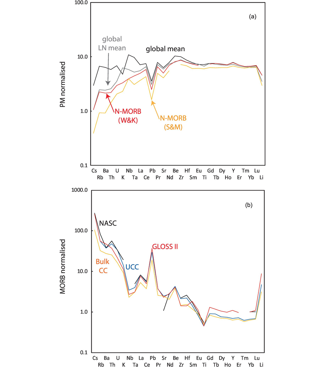
(a) Primitive mantle normalised plots for MORB (global mean, black line; White and Klein, 2014); MORB (global LN mean, grey line; Arevalo and McDonough, 2010); N-MORB (global mean, red line; White and Klein, 2014); and N-MORB (global mean, orange line; Sun and McDonough, 1989). The data are given in Table 4.9, columns 5–8. The normalising values are from the PM composition of Palme and O’Neill (2014) and given in Table 4.9, column 4. (b) MORB normalised plots of NASC (Gromet et al., 1984), upper continental crust (UCC) and bulk continental crust (bulk CC) (Rudnick and Gao, 2014) and GLOSS II (Plank, 2014). The data are given in Table 4.9, columns 9–12. The normalising values are from the global LN-MORB of Arevalo and McDonough (2010) given in Table 4.9, column 6.
4.4.1.3 MORB-Normalised Multi-element Diagrams
MORB normalised multi-element diagrams are most appropriate for evolved basalts, arc basalts, andesites, and the felsic rocks of the continental crust. The logic is that MORB normalisation is used to understand those rocks for which MORB might be the parental material. For the most part these are the rocks of the continental crust.
Four sets of normalising values are given in Table 4.9. The global MORB average of White and Klein (2014) represents the mean of 1975 MORB samples from all the major ocean basins, filtered for data quality. However, not all samples report values for all trace elements and their distribution is not Gaussian; therefore, it is recommended to use the log-normal mean values of Arevalo and McDonough (2010) (Table 4.9, column 6). N (‘normal’)-MORB is MORB which is depleted in highly incompatible elements and has a (La/Sm)N ratio of <1.0. N-MORB represents MORB which has not been influenced by mantle plumes (and thereby enriched). Two sets of N-MORB values are given in Table 4.9, that of White and Klein (2014) and the much-used values of Sun and McDonough (1989). The newer values of White and Klein (2014) are preferred since they are based upon more and better quality data.
4.4.1.4 Interpreting Multi-element Diagrams for Igneous Rocks
As an example of how to interpret multi-element diagrams, consider the primitive mantle normalised plot for N-MORB (Figure 4.20a). In this diagram trace element concentrations in N-MORB are characterised by a strong depletion of the most incompatible elements at the left side of the diagram, increasing to higher concentrations and a flatter trend for the more compatible elements on the right side of the diagram. Normalised values progressively increase from ~ 1× PM to about 8× PM with increasing compatibility; the more compatible high field strength (HFS) elements show a flat trend with values about 8× PM. In this particular order of the elements there are negative anomalies for Pb, Sr and Li. Concentrations in the global LN-MORB are similar, but values for the highly incompatible elements are higher and there is a small positive K anomaly. In contrast the trend for highly incompatible elements in the global mean is more erratic than for N-MORB and the global LN mean (Figure 4.20a). Despite the difference between these models of MORB, all averages show a strong pattern of incompatible element depletion, indicating that the MORB source has experienced previous melt extraction. The small anomalies for individual elements are thought to be a particular feature of the source.
A second example shows a MORB-normalised plot for the average composition of the bulk continental crust (Figure 4.20b). Here there is a pronounced decrease in element concentrations associated with increasing element compatibility during MORB melting. The most incompatible elements are present at more than 100× MORB, whereas the HFS element concentrations are generally similar to MORB, indicating the way in which incompatible elements tend to be fractionated into the continental crust. Significant deviations from this trend are the negative anomalies in the concentrations of Nb, Ta and Ti, which may represent the presence of a Ti-bearing phase in the source, and positive anomalies for Pb, Be and Li, which may reflect fluid-related processes. In more evolved felsic rocks, anomalies for specific elements may be controlled by individual minerals; for example, Zr concentrations may be controlled by zircon, P by apatite, the LREE and Th by allanite, HREE by garnet, Sr by plagioclase, and Ti, Nb and Ta by ilmenite, rutile or titanite (see Section 4.2.1.8).
4.4.2 Multi-element Diagrams for Clastic Sediments
The processes controlling the trace element composition of sedimentary rock may also be investigated using multi-element normalised diagrams, although they are not as widely used as their equivalents in igneous petrology. The most commonly used normalising values have been those for the North American shale composite (NASC) of Gromet et al. (1984) taken to represent ‘average crustal material’. However, the range of trace elements reported is small (see Table 4.9, column 9) and there are now better-quality data for more elements. For this reason, the average values for the upper continental crust or the bulk crust of Rudnick and Gao (2014) are preferred. An alternative is to use the average global subducting sediment (GLOSS) recently recalculated as GLOSS II by Plank (2014; Table 4.9, column 12) which is based on the average geochemical composition of subducting sediments. GLOSS II represents the average of 27 averages from each of the different subduction zone trenches. Trace element concentrations in GLOSS II are very similar to those for the upper continental crust (Figure 4.20b).
Multi-element diagrams for clastic sediments record information about the source of the sediment, continental weathering processes (seen in the concentrations of K, Rb, Cs, Li) and contributions from both biological (REE) and hydrothermal (Pb and REE) marine processes. This may be seen in GLOSS II where, although the shape of the pattern is similar to that of the bulk continental crust, some values are higher, indicating input from sources in addition to the crustal source, and others are lower, due to the dilution effect of a biological component (Plank 2014). The composition of GLOSS is also important for understanding large-scale subduction processes and may be used for tracing elements added to a subduction system through their input as sediments.
4.5 Diagrams Displaying Highly Siderophile Elements (HSE) and Platinum Group Elements (PGE)
The highly siderophile elements (HSE) include the elements Re, Os, Ir, Ru, Pt, Rh, Pd and Au. The platinum group elements (PGE), also known as the platinum group metals (PGM), are a subset of the HSE and include the elements Ru, Rh, Pd, Os, Ir and Pt. The PGE are known as the noble metals when they include Au. The PGE are divided on the basis of their geochemical behaviour into two subgroups:
Gold is often associated with the latter group. The concentrations of HSE in planetary materials and in rocks are extremely low. For example, in MORB, where concentrations are particularly low, they are reported in either parts per billion (ppb) or parts per trillion (ppt).
The HSE are particularly important in both cosmochemistry and mantle geochemistry. As the name indicates, they are siderophile and they show a strong affinity for the metallic iron phase. Thus, their concentrations in planetary bodies relate to the formation of an iron-rich metallic core. In the absence of metallic iron, they are strongly chalcophile and have a strong affinity for a sulphide phase. The basic data for the HSE, the melting temperature of the metals, the 50% equilibrium condensation temperatures (a function of processes), the metal–silicate partition coefficients, and concentrations in CI chondrites and the primitive mantle are given in Table 4.10.
| Element | Symbol | Atomic number | Melting temperature, K | 50% equilibrium condensation temperature, K | Metal–silicate D at 1 bar | CI chondrite Orgueil (ppm) | CI chondrite (ppm) | Primitive mantle (ppm) | Primitive mantle (ppm) |
|---|---|---|---|---|---|---|---|---|---|
| Reference | 1 | 1 | 1 | 1 | 2 | 1 | 2 | ||
| Rhenium | Re | 75 | 3453 | 1821 | 1.1 × 10⁵–2.8 × 10⁶ | 0.0381 | 0.040 | 0.00035 | 0.00035 |
| Osmium | Os | 76 | 3327 | 1812 | 1.5 × 10⁴–1.0 × 10⁶ | 0.4605 | 0.495 | 0.00390 | 0.00390 |
| Iridium | Ir | 77 | 2683 | 1603 | 2.1 × 10⁵–3.5 × 10⁷ | 0.4306 | 0.469 | 0.00350 | 0.00350 |
| Ruthenium | Ru | 44 | 2583 | 1551 | 1.3 × 10⁵–7.4 × 10⁶ | 0.6374 | 0.690 | 0.00700 | 0.00740 |
| Platinum | Pt | 78 | 2045 | 1408 | 3.7 × 10⁴–8.6 × 10⁵ | 0.8735 | 0.925 | 0.00760 | 0.00760 |
| Rhodium | Rh | 45 | 1826 | 1392 | 4.5 × 10⁴–1.6 × 10⁶ | 0.1310 | 0.132 | 0.00120 | 0.00120 |
| Palladium | Pd | 46 | 1825 | 1324 | 2.2 × 10³–2.0 × 10⁴ | 0.5705 | 0.560 | 0.00710 | 0.00710 |
| Gold | Au | 79 | 1337 | 1060 | 1.0 × 10³–5.0 × 10³ | 0.1750 | 0.148 | 0.00170 | 0.00170 |
4.5.1 The Application of the HSE in Cosmochemistry
In cosmochemistry the HSE can aid our understanding of the large-scale processes associated with planetary differentiation, in particular, the process of core formation. This is because of their strong affinity for metal relative to silicate. With the exception of Au all have higher melting temperatures than that of iron (1665 K) (Table 4.10). The Ir-group PGE are characterised by higher melting temperatures than the Pt-group PGE. When presented on element versus concentration diagrams the HSE are ordered according to their melting temperature with Re having the highest melting temperature to the left of the plot, through to Au with the lowest melting temperature on the right, and arranged in the order given in Table 4.10 (Figure 4.21a). The elements are separated with equal spacing, although not every study reports the full range of elements and Rh is frequently omitted. Concentrations are normalised using the measured values for CI chondrites (Table 4.10) and presented on a log scale (Figure 4.21a).
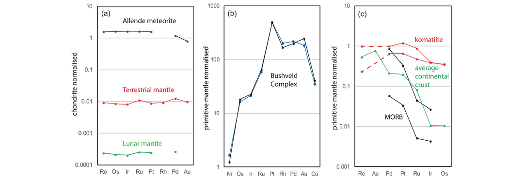
(a) CI-chondrite normalised plot for the HSE in the Allende meteorite, the lunar mantle and the Earth’s primitive mantle (Terrestrial mantle). CI normalising values from Day et al. (2016). Allende data, lunar mantle data and primitive terrestrial mantle data also from Day et al. (2016). Elements organized in order of decreasing melting temperature, left to right. (b) HSE data with Ni and Cu normalised to values for the primitive mantle for two PGE-rich samples from the Merensky Reef of the Bushveld Igneous Complex, South Africa. PM normalising values from Palme and O’Neill (2014), rock data from Barnes and Maier (2002). Elements organized in order of decreasing mantle compatibility, left to right. (c) HSE data for MORB (black lines, range from Rehkamper et al., 1999), komatiites in the Barberton greenstone belt, South Africa (red lines, from Puchtel et al., 2014) and the average bulk continental crust of Rudnick and Gao (2014) (green line). PM data from Palme and O’Neill (2014). Elements organized in order of increasing mantle compatibility, left to right. Note the different scales.
The distribution of the HSE in planetary materials can also be understood in terms of their temperature of condensation during the cooling of a solar nebula. This data is normally reported as the temperature at which 50% of the metal is condensed. The elements Re, Os, Ir, Ru, Pt and Rh are regarded as ultra-refractory because they have a very high condensation temperature and condense to refractory metal alloy grains. The elements Au and Pd are classified as moderately volatile with lower condensation temperatures. A further means of understanding the partitioning of elements during planetary formation and differentiation is through their metal–silicate partition coefficient, given in Table 4.10 for 1 bar of pressure.
4.5.2 The Application of the HSE in Mantle Geochemistry
In mantle geochemistry the HSE are treated slightly differently from in cosmochemistry, and in trace element variation diagrams the elements tend to be arranged according to their incompatibility in the silicate mantle. The sequence of increasing compatibility, from the most incompatible to those elements which are more compatible, is:
This is the order in which the elements will be concentrated during the partial melting of a purely silicate mantle. One measure of the degree of fractionation during partial melting is the ratio (Pd/Ir)N. This records the fractionation between one of the least compatible elements (Pd) relative to one of the more compatible elements (Ir).
Estimates of the composition of the primitive mantle are given in Table 4.10, and these can be used as an alternative to chondritic values for normalising mantle-derived melts. Compositional estimates of the primitive mantle are based upon the observation that Ir has a near uniform distribution in mantle peridotites. HSE ratios relative to Ir are then determined in fertile mantle peridotites (samples with high Al2O3), and calculated using the constancy of Ir concentrations. As noted above, HSE concentrations in the mantle are very low – about 100× less than chondrite – but are broadly chondritic (Figure 4.21a). Nevertheless, despite their very low concentrations their abundances are higher than those predicted from the process of core formation alone and imply the additional input of HSE into the Earth after core formation. This process is referred to as the addition of a late veneer of chondritic material to the Earth after core formation.
There are three important controls on HSE concentrations in melts during mantle melting. The first is the degree of partial melting. Day et al. (2016) showed that for the highly incompatible element Pd, concentrations increase in melts in parallel with the degree of melting, so that high-degree melts such as komatiites have higher concentrations of Pd than low-degree melts such as alkali basalts. A second control is the sulphur content of the source. In the absence of grains of metallic iron and PGE alloys, the HSE will be strongly partitioned into sulphides in the source. This effect will continue to be seen until the sulphide minerals in the source are completely melted out. A further control is mineralogical. The presence of PGE alloys and also chrome spinel in the source are both thought to exercise some control on HSE abundances in mantle melts and may govern the concentrations of Ir and Ru. However, the role of chrome spinel is complex, for a detailed examination shows that often the PGE are not present in solid solution but are present as inclusions of PGE alloys and oxides.
In MORB, HSE concentrations may be so low that some elements are below the limits of detection. In this case analyses may be limited to the elements Ir, Ru, Pt and Pd (e.g., Rehkamper et al., 1999; Bézos et al., 2005; Figure 4.21c). In MORB immiscible sulphide melts can be important in scavenging the PGE. In gabbros, particularly where they are associated with sulphides, concentrations of HSE are higher and may be present at the ppm level. In this case a wider range of HSE are reported along with Ni and Cu concentrations. For example, Barnes and Maier (2002) in their study of the Merensky Reef in the Bushveld Igneous Complex, South Africa, report the elements Ni, Os, Ir, Ru, Rh, Pt, Pd, Au and Cu (Figure 4.21b). The relevant normalising values for Ni are CI = 10,910 ppm and PM = 1860 ppm, and for Cu are CI = 133 ppm and PM = 20 ppm (data from Palme and O’Neill, 2014).
HSE data for komatiites, MORB and the continental crust are plotted according to their incompatibility in Figure 4.21c. In all cases the concentrations of the least compatible elements are the highest and decrease in the direction of the more compatible elements. This is clear in the MORB samples and indicates a strong control by partial melting. The affinity with the crustal pattern may suggest a relationship between MORB and the continental crust. In komatiites, the higher concentration of the more compatible elements may reflect higher degrees of melting of the HSE hosts.
4.6 Bivariate Trace Element and Trace Element Ratio Plots
Thus far in this chapter we have concentrated on the display of trace element data using different types of multi-element plot. This approach has the advantage of utilising a large number of elements and allowing broad conclusions to be drawn from their geochemical behaviour. However, multi-element plots have the disadvantage that only a few samples can be shown on a single diagram before it becomes cluttered and hard to read. In this case a bivariate plot showing elements or element ratios is preferred, in particular, when geochemical trends are sought. The principles behind variation diagrams have already been discussed in Section 3.3 with respect to major element geochemistry, and many of these principles also apply to trace elements plots.
4.6.1 The Selection of Trace Elements to Plot on Bivariate Graphs for Igneous Rocks
Many igneous rocks have had a complex history of solid–liquid equilibria in their journey from the source region to their site of emplacement. In addition, they may have interacted with fluids during or after their solidification. The task for the igneous geochemist, therefore, is to work out which trace elements are indicative of which processes in this complex history. The clues come from a knowledge of mineral-melt (and the lesser known mineral-fluid) partition coefficients and the physical laws which govern the concentrations of trace elements in igneous rocks. Most fruitful are trace elements which show extreme behaviour, such as the highly incompatible and the highly compatible elements. This is illustrated in general terms in Figure 4.22, in which the fractionation of selected trace and major elements between the continental crust, MORB and residual mantle is plotted against their partition coefficients (Hofmann, 2014).
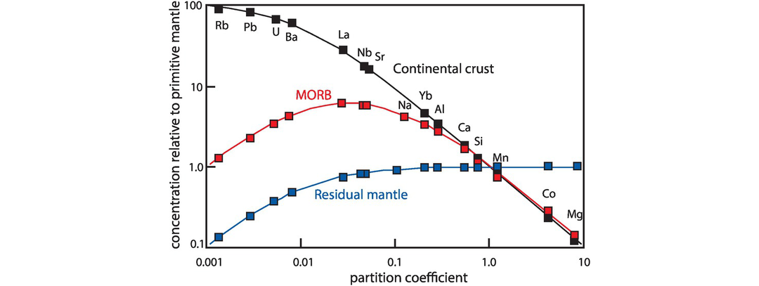
The abundances of selected trace and major elements in average continental crust, average MORB and residual mantle normalised to primitive mantle plotted relative to their partition coefficient.
Further clues may come from the inspection of multi-element plots, in particular, where trace element concentrations depart from otherwise smooth trends, for these elements may form the basis for identifying particular processes and in some instances even source characteristics. In this case it is instructive to plot the ratio of the anomalous element to an adjacent element which defines part of the overall smooth trend. However, care must be exercised in this process because some ‘anomalous’ trace element concentrations may be a function of the order in which the elements are plotted on the multi-element diagram. These trace elements or element ratios may then be used to determine variables such as the mechanism or style of melting, the degree of partial melting, the degree of fractional crystallisation and the composition and mineralogy of the source composition which has been melted. A similar approach is discussed by Pearce (2008) in which the logic used in selecting different trace elements to identify different magmatic process is carefully argued.
4.6.1.1 The Behaviour of the Highly Incompatible Elements
Highly incompatible element concentrations are particularly sensitive to partial melting processes when the degree of partial melting is low, as is illustrated in Figures 4.9a and 4.10a. The more incompatible an element is, the more sensitive it is to the degree of partial melting. This is true for both batch melting and fractional melting, but the effect is more extreme during fractional melting. This is illustrated with reference to the batch melting equation (Section 4.2.2.2, Eq. 4.6): when D is very small (D < 0.001), CL/Co reduces to 1/F. In other words, the concentration of a highly incompatible element in a melt relative to the source is inversely proportional to F, the degree of melting. Thus, when the melt fraction is small, all of the highly incompatible trace elements partition into the melt. A similar effect is seen during fractional crystallisation when the bulk partition coefficient of the fractionating phases is very small: at small fractions of melt remaining, CL/Co reduces to 1/F (Figure 4.13a). This effect is even more strongly marked in AFC processes (Figure 4.14).
It has also been shown that when D is very small, the ratio of two highly incompatible elements in a basaltic melt will mirror that of the source. For example, during batch melting, when D < 0.01, then CLelt-1/CLelt-2 = Coelt-1/Coelt-2 (see Hofmann et al., 1986; Arevalo and McDonough, 2010). This relationship is very powerful because it means that the ratio of a pair of highly incompatible elements whose bulk partition coefficients are very similar will not vary in the course of fractional crystallisation and will vary little during batch partial melting, and so allows us to ‘see through’ the effects of fractional crystallisation and through different degree of partial melting to identify the character of the source materials.
4.6.1.2 Estimation of Partition Coefficients from Trace Element Concentration Plots
Minster and Allegre (1978) showed that, from a rearrangement of the batch melting equation, a bivariate plot of the reciprocals of incompatible elements can be used to obtain information about partition coefficients during melting. Provided the mass fractions of the minerals in the melt remain constant, a linear trend on such a diagram characterises the batch melting process. Further, the slope and intercept of the trend can provide information about the difference in bulk partition coefficient between the two elements. If the samples are first normalised to the most enriched sample, elements with the same bulk partition coefficient will have a slope of 1 and an intercept of 0. If the bulk partition coefficients for the two elements change at different rates during melting, then a curvilinear trend will be produced (Bender et al., 1984). This approach was extended by Sims and DePaolo (1997) to show that log–log element plots are a useful way of assessing differences in D values between two incompatible elements. Elements with similar incompatibilities will plot as a straight line on a log–log plot (Figure 4.23), and where the incompatibility is identical the slope of the line will be unity. When the incompatible elements have differing D-values the slope will diverge from unity.
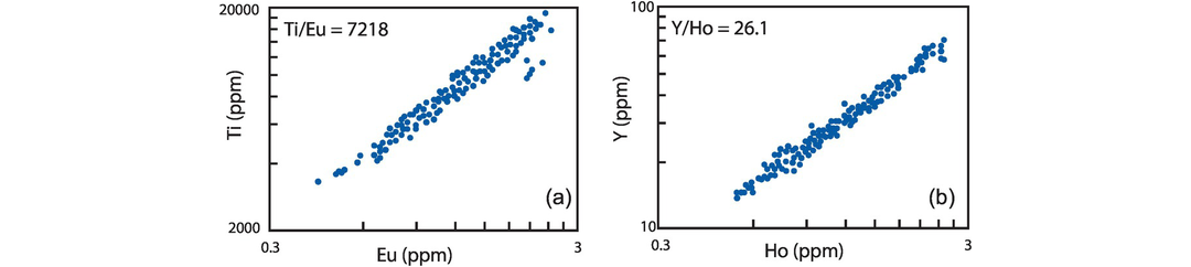
Log–log trace element plots for highly incompatible elements. (a) Ti versus Eu, and (b) Y versus Ho show the constancy of the respective trace element ratios (Ti/Eu = 7218 and Y/Ho = 26.1). These trace element ratios have been termed canonical trace element ratios and are thought to reflect the elemental ratios of the depleted mantle source.
4.6.1.3 Identification of Igneous Source Characteristics from Incompatible Element Ratio Plots
Authors working on oceanic basalts noted that some highly incompatible trace element ratios were constant regardless of the absolute concentrations of the elements present or the geographic location of the samples (e.g., Hofmann et al., 1986). Given their identical incompatibilities these ‘constant’ trace element ratios were termed canonical trace element ratios (Arevalo and McDonough, 2010; Hofmann, 2014) for they were thought to define the elemental ratios of the bulk silicate Earth (BSE). However, recent high-precision measurements on basalts from a range of MORB and ocean island basalt sources show the ratios vary between mantle sources and they are not indicative of the BSE. Instead, these trace element ratios are thought to reflect the trace element ratios of the individual sources of the different types of oceanic basalt (Arevalo and McDonough, 2010).
Early studies sought to demonstrate the constancy of trace element ratios using a plot in which a trace element ratio is plotted on the y-axis and the numerator of the ratio is plotted on the x-axis over a range of abundance. However, as discussed in Section 2.6, this type of plot can give rise to spurious self-correlation (see also Sims and DePaolo, 1997). A better alternative, therefore, is a plot of the trace element ratio versus MgO, in which MgO is a proxy for the fractionation index (Arevalo and McDonough, 2010), for this has the capacity to show the constancy of the ratio over a range of melt compositions. The most robust approach, however, as discussed in Section 4.6.1.2, is to use elemental log–log plots (Figure 4.23), for where these plots have a slope of 1, the elements have identical incompatibilities (Hofmann, 2014), and where the slope of the correlation line is not unity, the relative incompatibilities can be estimated.
In a detailed high-precision analytical study of 792 samples of MORB, Arevalo and McDonough (2010) showed that the ratios Ti/Eu, Y/Ho and Ce/Pb remain constant during MORB genesis and that these ratios reflect the composition of the MORB (depleted mantle) source (Figure 4.23). They showed that different ocean basins have sources with slightly different trace element ratios, raising the interesting question as to why this should be so. Conversely, the trace element ratios Ba/Th, Nb/U, Zr/Hf, Nb/Ta, Sr/Nd and Th/U, previously also thought to be indicative of the MORB source, are now known to fractionate during MORB genesis and do not faithfully record the composition of the depleted mantle.
4.6.1.4 Some Important Trace Element Ratios
There is a very large number of possible trace element ratios that can be plotted to summarise relationships in large geochemical data sets. A number of workers have sought to characterise the proposed mantle end-member compositions in terms of their trace element concentrations (Salters and Stracke, 2004; Willbold and Stracke, 2010; White and Klein, 2014). In addition, Rudnick and Gao (2014) provide a comprehensive review of the trace element composition associated with continental crust. Some values currently in use for highly incompatible trace element ratios which are immobile during metamorphism are given in Table 4.11. A selection of incompatible element ratios is described below with a particular emphasis on basaltic samples.
| Zr/Nb | La/Nb | Ba/Nb | Ba/Th | Rb/Nb | Th/Nb | Th/La | Ba/La | |
|---|---|---|---|---|---|---|---|---|
| Mantle | ||||||||
| DMa | 48.1 | 1.21 | 6.13 | 114 | 0.61 | 0.05 | 0.04 | 5.07 |
| HIMUb | 4.02 | 0.66 | 4.97 | 75.8 | 0.35 | 0.07 | 0.10 | 7.51 |
| EMIb | 6.36 | 1.3 | 14.9 | 173 | 0.97 | 0.09 | 0.07 | 11.8 |
| EMIIb | 4.53 | 0.98 | 10.7 | 79.5 | 0.83 | 0.13 | 0.14 | 10.9 |
| Continental crustc | ||||||||
| Upper | 16.1 | 2.6 | 52.0 | 59.4 | 7.0 | 0.88 | 0.34 | 20.1 |
| Middle | 14.9 | 2.4 | 53.2 | 81.8 | 6.5 | 0.65 | 0.27 | 22.2 |
| Lower | 13.6 | 1.6 | 51.8 | 216 | 2.2 | 0.24 | 0.15 | 32.4 |
The trace element ratio of the light REE elements (La/Sm)N is particularly useful in classifying MORB samples, for while these are typically depleted in the light REE, some are enriched. The ratio (La/Sm)N is a useful measure of light REE depletion, and samples with (La/Sm)N > 1.0 are classified as E-MORB (enriched MORB), whereas those with (La/Sm)N < 1.0 are classified as N-MORB (normal MORB). These differences may be shown on REE plots, but they can be helpfully summarised on a (La/Sm)N versus La trace element plot. A similar distinction is useful in examining some mantle peridotites to show the extent to which they may have been depleted and/or re-fertilised (Figure 4.24).
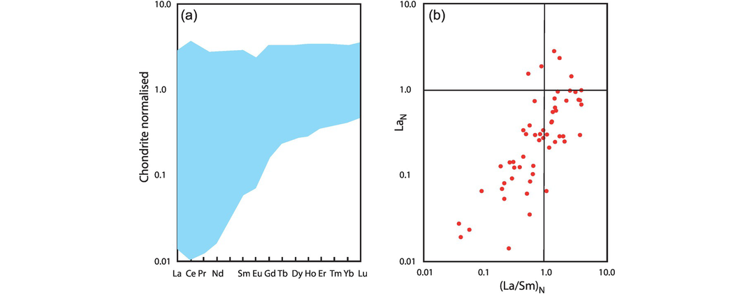
REE data for ocean floor mantle peridotites. (a) REE patterns show a wide range of patterns, some of which show extreme depletion in the light REE; (b) the same data presented as (La/Sm)N versus LaN.
Trace elements with identical charge and ionic size are expected to behave in an identical manner and the ratios of the trace element pairs Nb/Ta and Zr/Hf in all terrestrial rocks should be similar to that in chondritic meteorites (Nb/Ta = 18.9; Zr/Hf = 34.1; Palme and O’Neill, 2014). However, this is not always the case, demonstrating that these trace element ratios have the power to identify petrological processes. For example, Niu and Batiza (1997) showed that the two ratios vary significantly in seafloor basaltic lavas from seamounts near the axis of the East Pacific Rise, and Foley et al. (2002), in a study on the origin of felsic continental crust, exploited the differences in the Nb/Ta ratio between oceanic basalt and Archaean continental crust to argue for an amphibolite melting model for early continental crust.
The K/U ratio is important in constraining the Earth’s heat budget and noble gas abundances in the primitive Earth. One approach to resolving these first-order issues is to measure the K/U of MORBs, for, given that K and U behave similarly during partial melting and crystal fractionation, these provide a window into the K/U of the upper mantle. Arevalo et al. (2009) reported a K/U ratio for MORB of 19,000, but found that this differed from the ratio in ocean island basalts. However, given the potential for the mobility of these elements, the measurements need to be determined on fresh basaltic glass.
It can be helpful to compare the trace element ratios between major crustal reservoirs. For example Nb/Th is ~1.4 in average continental crust, ~15.7 in MORB, and 7–8 in the primitive mantle, indicating that there has been significant fractionation during the formation of MORB and the continental crust. These differences were exploited by Pearce (2008) in an attempt to identify mantle–continental crust interaction in basaltic magmas. In this study, Pearce normalised the Nb/Th ratio using Yb, to minimise the effects of fractional crystallisation and on the resulting Th/Yb–Nb/Yb plot identified a mantle array which encompasses the full range of MORB and ocean island basalt compositions (Figure 4.25). In a similar way, Fitton et al. (1997) used the incompatible element ratios Nb/Y and Zr/Y to show the differences between plume and N-MORB mantle sources, and Condie (2005) proposed that incompatible element ratios Zr/Nb, Nb/Th, Zr/Y and Nb/Y can be used to characterise the mantle source of tholeiitic basalts.
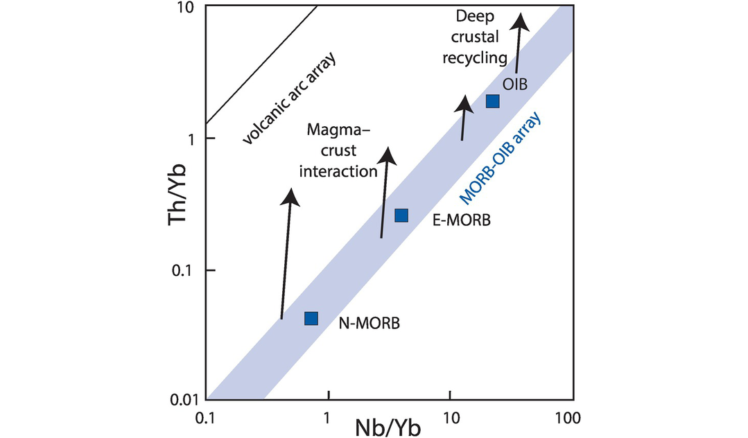
Nb/Yb versus Th/Yb diagram showing the MORB-OIB (ocean island basalt) mantle array (shaded area) and the compositions of average normal MORB (N-MORB), average enriched MORB (E-MORB) and average ocean island basalt (OIB). Volcanic arc basalts plot above the mantle array. The effects of magma–crust interaction and deep crust recycling are indicated by the arrows.
4.6.1.5 Applications to Felsic Rocks
Identifying similar ‘canonical’ trace element ratios in felsic rocks (and thus their source characteristics) is much more difficult than in mafic rocks. This is because felsic melts are often highly fractionated and/or modified by fluid mobility. Further, the fractionation of minor phases such as apatite, zircon, monazite, titanite and ilmenite modifies many of the critical trace element ratios to the extent that it is impossible to determine the nature of the source using this method.
However, some trace element ratios can be used to evaluate large-scale mass balance models involving felsic crust. This is because some highly incompatible element ratios are very different in the continental crust from the mantle. For example, Arevalo and McDonough (2010) use the ratios Y/Ho and Th/U to demonstrate the complementarity of the continental crust and depleted mantle relative to a chondritic source (although this is not consistent with the result from Ti/Eu and Nb/Ta ratios). Similarly, Collerson and Kamber (1999) used the changing ratio of Nb/Th in mantle rocks over time to evaluate the extraction of the continental crust from the Earth’s mantle.
4.6.1.6 Compatible Element Plots
Compatible trace element concentrations change dramatically in an igneous liquid during fractional crystallisation (Figure 4.13a). Thus, bivariate plots of compatible elements, plotted against an index of fractionation (e.g., MgO) can be used as a test for fractional crystallisation. The effect is less marked during in situ crystallisation except for the case when a large melt fraction is returned to the magma chamber (Figure 4.13d). Compatible elements are also strongly depleted during AFC processes when the rate of assimilation is high and the trace element concentration in the wall rock is less than in the melt (Figure 4.14).
During low and moderate degrees of partial melting the concentrations of highly compatible elements in the source are buffered by the solid phases present. This means that even if the source has undergone prior partial melting, trace element concentrations will remain largely unchanged during both batch (Figure 4.9b) and fractional (Figure 4.10b) melting.
4.6.2 Bivariate Plots in Sedimentary Rocks
Bivariate trace element plots in sedimentary rocks are mostly used to detect mixing processes in sediments. Norman and De Deckker (1990) suggest that linear correlations amongst a diverse group of elements over a broad range of concentrations may indicate mixing of two sedimentary components, although major element plots can also be used to discern this process (Figure 3.13). A more complete discussion of bivariate trace element plots in sediments is given in Section 5.5.3.
4.7 Enrichment–Depletion Diagrams
Enrichment–depletion diagrams are a convenient way of showing relative enrichment and depletion in trace (or major) elements as a ‘positive–negative’ histogram. Diagrams of this type can be useful for demonstrating the extent of elemental enrichment or depletion in an igneous suite by comparing the chemistries of early and late members of a series. Hildreth (1981) compared the relative concentrations of the early and late members of Bishop Tuff (Figure 4.26). The x-axis of the graph shows the elements arranged by atomic number and the y-axis the concentration of an element in the latest erupted ejecta divided by concentrations for the earliest erupted ejecta. The values on the y-axis may also be presented on a logarithmic scale.
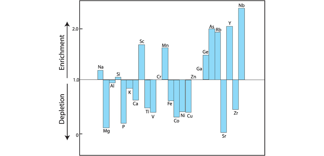
Enrichment–depletion histogram. The enrichment factors for selected major and trace elements from Bishop Tuff are arranged in order of increasing atomic number. The diagram compares the concentrations of the late members relative to the early members of Bishop Tuff and is thought to be a measure of the zonation of the magma chamber.
Enrichment–depletion diagrams are also useful as a way of displaying element mobility. This has been used particularly in alteration zones associated with hydrothermal mineralisation. For example, Taylor and Fryer (1980) show the relative mobility of trace and major elements in the zones of potassic and propylitic alteration associated with a porphyry copper deposit. In this case the enrichment/depletion is measured relative to the composition of the unaltered country rock. In a similar way, enrichment–depletion diagrams may be used in the study of compositional change during rock weathering such that the composition of the weathered product can be shown relative to the composition of the original rock.
4.8 Modelling Trace Element Processes in Igneous Rocks
One of the most important uses of trace elements in modern igneous petrology is in the testing of hypotheses through the modelling of geochemical processes. This frequently involves constructing a geochemical model which is thought to represent the processes which have taken place and then comparing the model results with those of the actual measurements (Allègre and Minster, 1978; Shaw, 2006). Trace element modelling depends upon the mathematical expressions which describe the equilibrium partitioning of trace elements between minerals and melt during igneous processes (Section 4.2.2) and a precise knowledge of trace element partition coefficients (Section 4.2.1 and Tables 4.1–4.4). For successful geochemical modelling, three conditions should be fulfilled. First, trace element concentrations must be determined with great accuracy; otherwise, it is impossible to discriminate between competing hypotheses (Arth, 1976). Second, partition coefficients for the conditions under which the process is being modelled must be known accurately. Third, the starting composition must be known. This last condition is not always fulfilled and sometimes a reasonable assumption of the starting composition must be made which is later refined as the model is developed.
The ultimate aim of geochemical modelling is to determine the processes operating within a given suite of rocks. Often this is at a local scale, such as in an individual magma chamber, or at a regional scale, such as a volcanic province; but such is the power of geochemistry that in some instances it can be about large-scale reservoirs, such as the whole of the continental crust or the entire depleted upper mantle.
As previously discussed, many igneous rocks have evolved through a range of processes and each of these may need to be determined separately and if necessary ‘stripped away’ in order to reveal underlying processes. An extreme example would be a suite of rocks in which first the effects of element mobility have to identified and the relevant samples removed from the data set. Then the effects of crystal fractionation identified and the least fractionated samples isolated. The remaining samples can then be used to identify the conditions of partial melting and ultimately the nature of the source.
It is important to note that geochemical models do not necessarily provide a unique solution to a geological problem. Uncertainty about the precise initial composition of the source or the melt, the correct partition coefficients and the precise physical processes of melting and/or fractionation may mean that multiple solutions can fit the observed data. For this reason trace element modelling often has to be constrained by other data. These may be geochemical – major element or isotopic data, the results of experimental petrology, or field and petrographic observations. Often when these additional external constraints are introduced, reasonable assumptions can be made about the nature of the process being investigated. Allegre and Minster (1978) use the example of a suite of alkali basalts, for which they made the assumptions that they were formed by a small degree of partial melting of typical mantle material. These two assumptions, limiting the composition of the source and the range of F, simplified subsequent trace element modelling.
The results of trace element modelling calculations are plotted on a bivariate or multivariate graph and compared with an observed trend of measured rock compositions. This process is often carried out using a computer package such as t-IgPet (Carr and Gazel, 2017), Petrograph (Petrelli et al., 2005), or WinRock (Kanen, 2004). There is also the substantial work by Janousek et al. (2016) whose software is written using the R language. Here we illustrate modelling using the results of calculations in a spreadsheet so that the methodology is transparent. Initially, in Section 4.8.1 we discuss forward modelling in which model calculations are compared with the observed data, and then we consider inverse modelling where the data themselves can be used to constrain the model (Section 4.8.3).
4.8.1 Vector Diagrams
Changes in trace element concentrations may be modelled on a bivariate plot using vectors to show the amount and direction of change which will take place as a consequence of a particular process. Diagrams of this type are useful for quantifying the extent either of fractional crystallisation or of partial melting. For example, mineral vectors can be calculated to show the evolving composition of a melt in response to the removal of a fractionating mineral phase or mineral assemblage (Figure 4.27). The effects of fractionation calculated using the Rayleigh equation (Eq. 4.20) for plagioclase, clinopyroxene, orthopyroxene, hornblende, biotite and orthoclase from a granitic melt are shown in Figure 4.27. Partial melting vectors may be calculated in a similar way using the appropriate equations, to show changing melt or source compositions during the partial melting of a given source composition and mineralogy. The effects of different melting models, source compositions and mineralogy may be all explored in this way.
Thus, vector diagrams can be used to identify a fractionating phase on a bivariate plot. If, for example, on a plot of Ba versus Sr, the rock compositions define a liquid trend which could have been produced by crystal fractionation, then the slope of the trend can be compared with a mineral vector diagram (Figure 4.27) and the phase responsible for the fractional crystallisation trend can be identified. In addition, it is possible from the compositional range of the two elements to make an estimate of the amount of fractional crystallisation that has taken place. When there is more than one fractionating phase present, a composite vector can be calculated, although when this is the case it is not always possible to find a unique composition for the fractionating mineral assemblage. Although vector diagrams select only two out of a vast array of possible elements, they have the advantage of being able to display data from a large number of samples. This means that it is possible to view trends in the data. Consequently, both mineral and partial melting vectors can be plotted alongside observed trends on bivariate plots in order to identify possible magmatic processes.
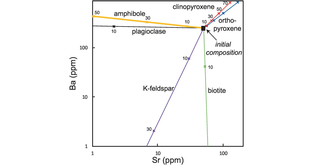
Vector diagram for Ba versus Sr (ppm). The figure shows the effects of Rayleigh fractionation of a felsic melt with an initial composition of 250 ppm Ba and 50 ppm Sr. Fractionation trends are shown for the phases orthopyroxene, clinopyroxene, plagioclase, amphibole, K-feldspar and biotite. The tick marks on the fractionation curves show the effects of 10, 30, 50 and 70% fractionation. The partition coefficient values for Sr and Ba are from Table 4.3. Note the logarithmic scale.
4.8.2 Modelling on Multivariate Diagrams
In this section we illustrate the way in which trace element modelling has been used to identify different petrogenetic processes in igneous rocks. Multivariate diagrams such as REE plots and multi-element diagrams can be used for petrogenetic modelling, although these are unable to clearly show more than a few samples on a single diagram. In this case the same operation is performed on each element in the plot and the resultant data array is compared with a measured rock composition. The process is illustrated in Figure 4.28 to show the effects of partial melting of a primitive mantle source (Figure 4.28a, b) and of olivine fractionation on a basaltic liquid (Figure 4.28c).
4.8.2.1 Partial Melting
An example of the behaviour of the REE during the partial melting of a mantle source to produce a basaltic melt is given in Table 4.12 and the results shown graphically (Figure 4.28). In this model all the results are chondrite normalised using the values of Barrat et al. (2012) (Table 4.7). The starting composition is the primitive mantle composition of Palme and O’Neill (2014) and this melting model is therefore more directly applicable to basaltic compositions in the Archaean. Two sets of partition coefficients are chosen to illustrate the way in which even the choice of partition coefficient may influence the outcome of geochemical modelling. On the left side of Table 4.12 the partition coefficients from Table 4.1 are used and on the right side of Table 4.12 the values of Bédard (2005, 2014) are used. It should be noted that the values for clinopyroxene are different in the two data sets, and since these values are much higher than those for olivine or orthopyroxene, they strongly influence the value of the calculated bulk partition coefficient D.
| Partition coefficients from Table 4.1 | Partition coefficients from Bédard (2005, 2014) | |||||||||||||||||
|---|---|---|---|---|---|---|---|---|---|---|---|---|---|---|---|---|---|---|
| Olivine | Ortho pyroxene | Clino pyroxene | Spinel | D | Olivine | Ortho pyroxene | Clino pyroxene | Spinel | D | |||||||||
| 50% | 40% | 8% | 2% | 50% | 40% | 8% | 2% | |||||||||||
| La | 0.0000 | 0.0008 | 0.0860 | 0.0000 | 0.0072 | La | 0.0002 | 0.0012 | 0.0900 | 0.0000 | 0.0078 | |||||||
| Ce | 0.0000 | 0.0016 | 0.1750 | 0.0000 | 0.0147 | Ce | 0.0004 | 0.0020 | 0.1600 | 0.0000 | 0.0138 | |||||||
| Pr | 0.0001 | 0.0032 | 0.2890 | 0.0000 | 0.0244 | Pr | 0.0008 | 0.0034 | 0.2000 | 0.0000 | 0.0178 | |||||||
| Nd | 0.0002 | 0.0056 | 0.4700 | 0.0000 | 0.0399 | Nd | 0.0012 | 0.0054 | 0.2800 | 0.0000 | 0.0252 | |||||||
| Sm | 0.0006 | 0.0150 | 0.8100 | 0.0000 | 0.0711 | Sm | 0.0026 | 0.0118 | 0.4000 | 0.0000 | 0.0380 | |||||||
| Eu | 0.0012 | 0.0300 | 1.0000 | 0.0000 | 0.0926 | Eu | 0.0051 | 0.0163 | 0.3300 | 0.0000 | 0.0355 | |||||||
| Gd | 0.0018 | 0.0340 | 1.0400 | 0.0000 | 0.0977 | Gd | 0.0050 | 0.0215 | 0.5000 | 0.0000 | 0.0511 | |||||||
| Tb | 0.0028 | 0.0540 | 1.2200 | 0.0000 | 0.1206 | Tb | 0.0067 | 0.0285 | 0.6000 | 0.0000 | 0.0628 | |||||||
| Dy | 0.0040 | 0.0770 | 1.4000 | 0.0000 | 0.1448 | Dy | 0.0089 | 0.0371 | 0.7000 | 0.0000 | 0.0753 | |||||||
| Ho | 0.0064 | 0.1000 | 1.3500 | 0.0000 | 0.1512 | Ho | 0.0115 | 0.0468 | 0.6700 | 0.0000 | 0.0781 | |||||||
| Er | 0.0110 | 0.1200 | 1.3400 | 0.0000 | 0.1607 | Er | 0.0143 | 0.0573 | 0.6500 | 0.0000 | 0.0821 | |||||||
| Tm | 0.0140 | 0.1700 | 1.3800 | 0.0000 | 0.1854 | Tm | 0.0172 | 0.0683 | 0.6600 | 0.0000 | 0.0887 | |||||||
| Yb | 0.0188 | 0.2200 | 1.4200 | 0.0000 | 0.2110 | Yb | 0.0203 | 0.0794 | 0.6800 | 0.0000 | 0.0963 | |||||||
| Lu | 0.0280 | 0.2200 | 1.1600 | 0.0000 | 0.1948 | Lu | 0.0233 | 0.0903 | 0.6800 | 0.0000 | 0.1022 | |||||||
| Batch modal partial melting | ||||||||||||||||||
|---|---|---|---|---|---|---|---|---|---|---|---|---|---|---|---|---|---|---|
| F | 0.05 | 0.10 | 0.15 | 0.20 | 0.25 | F | 0.05 | 0.10 | 0.15 | 0.20 | 0.25 | |||||||
| PM-normalised | PM-normalised | |||||||||||||||||
| 57 | La | 2.907 | 51.138 | 27.301 | 18.621 | 14.129 | 11.383 | 57 | La | 2.907 | 50.657 | 27.170 | 18.563 | 14.097 | 11.364 | |||
| 58 | Ce | 2.922 | 45.699 | 25.809 | 17.983 | 13.798 | 11.194 | 58 | Ce | 2.922 | 46.292 | 25.987 | 18.064 | 13.843 | 11.221 | |||
| 59 | Pr | 2.920 | 39.877 | 23.933 | 17.097 | 13.299 | 10.881 | 59 | Pr | 2.920 | 43.662 | 25.174 | 17.685 | 13.631 | 11.088 | |||
| 60 | Nd | 2.890 | 32.863 | 21.259 | 15.711 | 12.460 | 10.323 | 60 | Nd | 2.890 | 39.107 | 23.565 | 16.863 | 13.129 | 10.749 | |||
| 62 | Sm | 2.841 | 24.167 | 17.324 | 13.500 | 11.060 | 9.366 | 62 | Sm | 2.841 | 32.991 | 21.168 | 15.584 | 12.331 | 10.201 | |||
| 63 | Eu | 2.841 | 20.594 | 15.497 | 12.423 | 10.367 | 8.894 | 63 | Eu | 2.841 | 33.948 | 21.538 | 15.772 | 12.441 | 10.272 | |||
| 64 | Gd | 2.842 | 19.902 | 15.124 | 12.196 | 10.218 | 8.792 | 64 | Gd | 2.842 | 28.842 | 19.469 | 14.693 | 11.799 | 9.858 | |||
| 65 | Tb | 2.867 | 17.422 | 13.748 | 11.354 | 9.670 | 8.421 | 65 | Tb | 2.867 | 26.153 | 18.320 | 14.098 | 11.458 | 9.650 | |||
| 66 | Dy | 2.850 | 15.195 | 12.374 | 10.437 | 9.024 | 7.948 | 66 | Dy | 2.850 | 23.452 | 16.988 | 13.318 | 10.952 | 9.300 | |||
| 67 | Ho | 2.822 | 14.570 | 11.951 | 10.130 | 8.791 | 7.764 | 67 | Ho | 2.822 | 22.724 | 16.572 | 13.041 | 10.751 | 9.144 | |||
| 68 | Er | 2.822 | 13.923 | 11.535 | 9.846 | 8.588 | 7.615 | 68 | Er | 2.822 | 22.050 | 16.229 | 12.840 | 10.622 | 9.057 | |||
| 69 | Tm | 2.818 | 12.462 | 10.560 | 9.161 | 8.090 | 7.243 | 69 | Tm | 2.818 | 20.985 | 15.668 | 12.501 | 10.399 | 8.902 | |||
| 70 | Yb | 2.842 | 11.346 | 9.802 | 8.628 | 7.705 | 6.961 | 70 | Yb | 2.842 | 20.083 | 15.222 | 12.256 | 10.257 | 8.819 | |||
| 71 | Lu | 2.879 | 12.249 | 10.458 | 9.124 | 8.091 | 7.269 | 71 | Lu | 2.879 | 19.579 | 15.000 | 12.157 | 10.220 | 8.815 | |||
| Fractional crystallisation of olivine | ||||||||||||||||||
|---|---|---|---|---|---|---|---|---|---|---|---|---|---|---|---|---|---|---|
| F | 0.90 | 0.80 | 0.70 | 0.60 | 0.50 | |||||||||||||
| 15% batch modal melt | ||||||||||||||||||
| 57 | La | 18.621 | 20.690 | 23.276 | 26.601 | 31.034 | 37.241 | |||||||||||
| 58 | Ce | 17.983 | 19.981 | 22.478 | 25.689 | 29.970 | 35.964 | |||||||||||
| 59 | Pr | 17.097 | 18.997 | 21.371 | 24.424 | 28.494 | 34.192 | |||||||||||
| 60 | Nd | 15.711 | 17.457 | 19.638 | 22.443 | 26.183 | 31.418 | |||||||||||
| 62 | Sm | 13.500 | 15.000 | 16.873 | 19.282 | 22.493 | 26.989 | |||||||||||
| 63 | Eu | 12.423 | 13.802 | 15.525 | 17.740 | 20.693 | 24.826 | |||||||||||
| 64 | Gd | 12.196 | 13.549 | 15.239 | 17.412 | 20.308 | 24.362 | |||||||||||
| 65 | Tb | 11.354 | 12.612 | 14.183 | 16.204 | 18.896 | 22.664 | |||||||||||
| 66 | Dy | 10.437 | 11.591 | 13.034 | 14.888 | 17.359 | 20.815 | |||||||||||
| 67 | Ho | 10.130 | 11.248 | 12.644 | 14.438 | 16.828 | 20.170 | |||||||||||
| 68 | Er | 9.846 | 10.927 | 12.277 | 14.010 | 16.317 | 19.542 | |||||||||||
| 69 | Tm | 9.161 | 10.164 | 11.416 | 13.022 | 15.160 | 18.146 | |||||||||||
| 70 | Yb | 8.628 | 9.568 | 10.740 | 12.243 | 14.243 | 17.033 | |||||||||||
| 71 | Lu | 9.124 | 10.108 | 11.334 | 12.904 | 14.990 | 17.897 | |||||||||||
The melting model is based upon a primitive mantle mineralogy with 50% olivine, 40% orthopyroxene, 8% clinopyroxene and 2% spinel. Two different models are illustrated: (i) modal batch melting is shown for 5%, 10%, 15%, 20% and 25% melting (Figure 4.28a), and (ii) accumulated fractional melting for 1%, 2%, 5%, 10% and 15% melting (Figure 4.28b). The results using the partition coefficients from Table 4.1 are shown in black (the steeper REE trends), while results using the partition coefficients from Bédard (2005, 2014) are shown in red (the flatter REE trends) for both melting models (Figure 4.28a, b).
These results are summarised using (La/Yb)N versus LaN to show the degree of REE fractionation (Figure 4.28d). It is clear that the degree of fractionation of the REE (the (La/Yb)N ratio) is dependent on both the mechanism of melting and on the choice of partition coefficient.
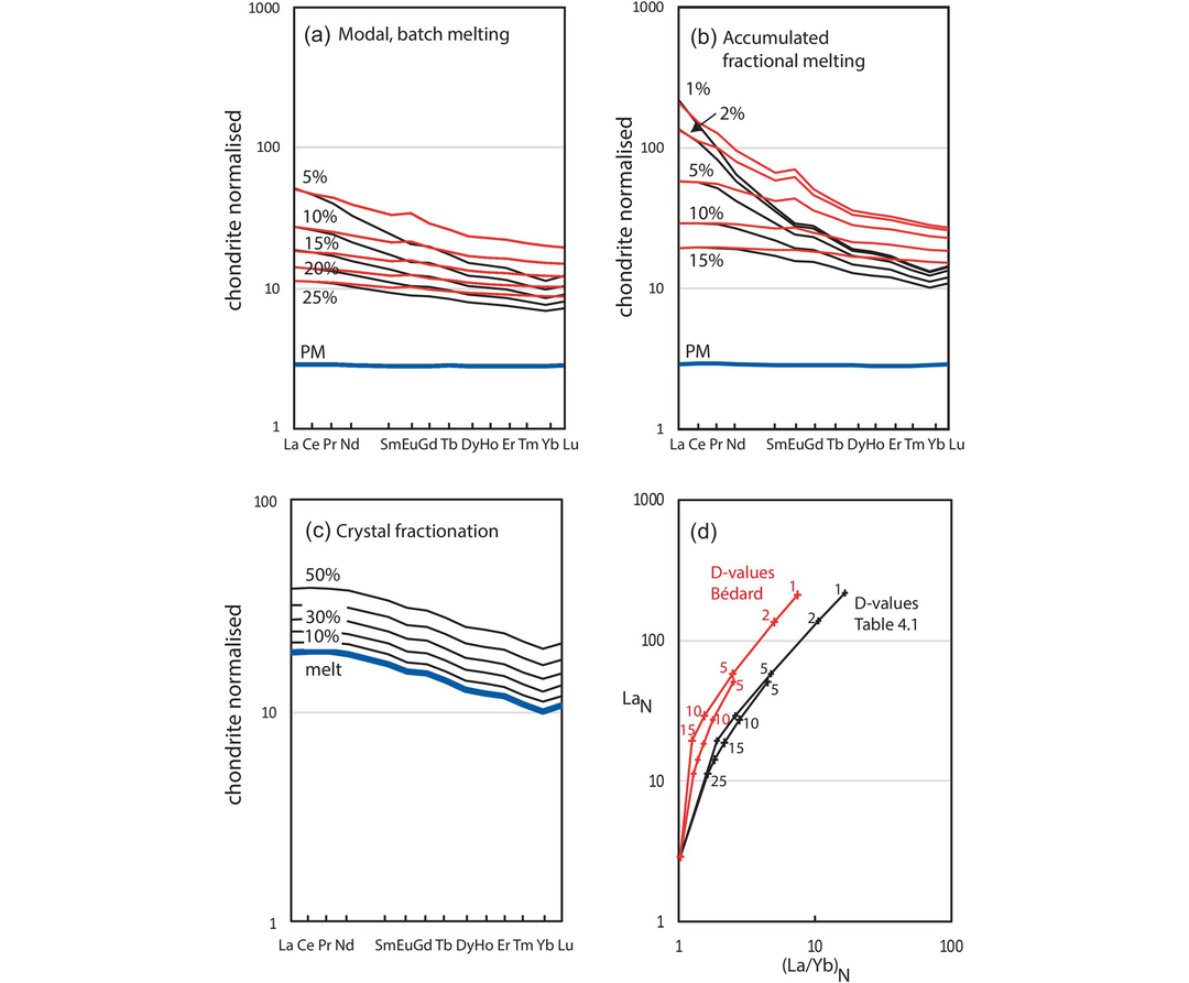
Geochemical modelling using REE. (a) REE plot showing the results of 5–25% modal batch melting of a primitive mantle composition. (b) REE plot showing the results of 1–15% accumulated fractional melting of a primitive mantle composition. (c) REE plot showing the results of 10–50% olivine fractionation in a basaltic melt produced by 15% modal batch melting of primitive mantle using partition coefficient data from Table 4.1. (d) (La/Yb)N versus LaN summarising the change in REE composition for the models presented in panels (a) and (b). The longer curves show the results of accumulated fractional melting and the shorter curves the result of modal batch melting. The numbers by the curves show the fraction of melting. In all panels the compositions shown as black lines use the partition coefficient data from Table 4.1, and those shown as red lines use the partition coefficient data of Bédard (2005, 2014). Further details are given in Table 4.12 and in the text.
4.8.2.2 Crystal Fractionation
A worked example of the behaviour of the REE during fractional crystallisation is given in Table 4.12 and illustrated in Figure 4.28c. In this example the starting composition is the 15% melt of primitive mantle formed during batch modal melting, calculated in Table 4.12. The effect on REE concentrations by the removal of 10%, 20%, 30%, 40% and 50% olivine (F = 0.9 to 0.5) using the olivine partition coefficients from Table 4.1 is shown (Figure 4.28c). It is clear that in this model, because of the highly incompatible nature of the REE in olivine, the REE concentrations in the melt increase, but the overall shape of the REE pattern does not change from that of the parental melt. Hence the (La/Yb)N ratio of the melt does not change even though the La content of the melt does.
4.8.2.3 Crustal Contamination and AFC Processes
Komatiitic magmas are thought to have had exceptionally high liquidus temperatures and often to have been contaminated with continental crust leading to the formation of basaltic komatiites. Geochemical support for this hypothesis comes from the enhanced ratios of trace elements such as Nb/La and La/Sm which correlate with Nd–isotopic compositions (Arndt et al., 2008). Arndt and Jenner (1986) calculated the compositional change in a komatiite from the Kambalda greenstone belt contaminated with a mixture of sediment and basalt using AFC modelling for major and trace elements.
One of the difficulties in recognising crustal contamination is that it is not always clear whether the ‘contamination’ has taken place in the crust or is a property of the mantle source, perhaps reflecting some very ancient modification of a mantle source with either subducted basalt or subducted sediment. Thus, Hughes et al. (2014) modelled AFC processes on a multi-element diagram for the contamination of primary mantle melts with Archaean continental crust. In this case the study suggests that crustal contamination was not a major contributor to the magmatic processes under consideration and that the trace element variability was a function of the mantle source compositions involved.
4.8.2.4 Open System Processes
Open system behaviour in magma chambers has been described in some detail in Section 4.2.2.3. However, the early work of O’Hara and Matthews (1981) and later studies such as that of Wooden et al. (1993), Fowler et al. (2004), and Heinonen et al. (2019) make it clear that fractional crystallisation in an open system is often accompanied by AFC processes as the magma reacts with the walls of the magma chamber in either the deep crust or the shallow continental crust. O’Hara and Matthews (1981) explored in some detail the behaviour of trace elements in an RTF magma chamber. They show the contrasting behaviour of incompatible and highly incompatible elements and show that potentially open system fractional crystallization is far more efficient in changing the ratio of incompatible and highly incompatible elements than is closed system fractional crystallization. Using chondrite normalised values of Ce/Yb to represent the slope of the REE diagram and Sm values as a measure of REE concentrations, they show on a bivariate plot of normalised Ce/Yb versus Sm the effects of the RTF process on partial melts of a variety of mantle sources coupled with crystal fractionation.
Recognising RTF processes in a lava sequence requires a very detailed and complete geochemical section. In a study of Oligocene andesites and basalts from southwest Idaho, USA, Norman and Leeman (1990) recognised a cyclicity in the trace and major element chemistry going up the stratigraphic section. On bivariate Ba–Sc and Th–Sc plots they showed that the scatter in the data cannot be accommodated by calculated fractional crystallisation and AFC trends alone, and required the addition of more mafic magmas during evolution of the magma chamber.
4.8.2.5 Magma and Source Mixing
A set of general mixing equations given by Langmuir et al. (1978) can be used to identify magma mixing and mixing in an igneous source region. These equations predict that mixing between two elements produces a straight line, whereas mixing between an element and an element ratio or between two ratios produces an asymptotic curve.
These two types of mixing (magma mixing and source mixing) can be differentiated by using differences in behaviour between compatible and incompatible elements. For example, since highly incompatible element ratios do not change during partial melting or fractional crystallisation, a mixing curve based upon incompatible element ratios is ambiguous, indicating either magma mixing or source mixing. Compatible elements ratios, on the other hand, are strongly fractionated during partial melting but will not reflect the ratios of the source region. Thus, if mixing is in the source region a compatible element plot will show a scattered trend, whereas the mixing of two melts will produce a simple mixing line.
4.8.3 Inversion Techniques Using Trace Elements
Trace element inversion techniques make use of the trace element composition of a mineral or melt to calculate the composition of the parental material – in the case of a mineral this is the melt from which it has crystallised, or in the case of a melt, it is the mineralogy and composition of the source from which it was derived. Inversion techniques require both the precise measurement of trace element concentrations in the mineral or melt to be investigated and a good knowledge of mineral-melt partition coefficients. In their most simple form, inversion methods use the mineral-melt partition coefficient equation (Eq. 4.3) and solve for either the melt composition if the composition of the solid phase is known or the solid phase if the melt composition is known. More detailed approaches utilise the trace element partitioning equations discussed in Section 4.2.2, although if not all the unknowns are determined some assumptions have to be made during the modelling.
The original methodology of trace element inversion was developed in a series of papers by Allegre et al. (1977), Minster et al. (1977), Allegre and Minster (1978), and Minster and Allegre (1978). These authors made use of the variability in elemental concentrations in a suite of cogenetic igneous rocks to determine unknowns such as the composition and mineralogy of the source, the physical process causing these variations (crystal fractionation, partial melting or other process), and the degree of partial melting or crystal fractionation. More recent mathematical inversion formulations for fractionation and partial melting processes have been given in Janousek et al. (2016), although are unhelpfully termed ‘reverse’ methods.
Inverse methods can in principle be applied to all petrological processes, although only fractional crystallisation and melting models are illustrated here. A first step in using the inverse approach for the study of trace elements is to attempt to identify the likely physical process which accounts for the variation in the data. This may be done by plotting selected trace elements on bivariate plots. For example, elements which are compatible will vary drastically in concentration during fractional crystallisation, while highly incompatible elements will vary most in abundance during partial melting. In addition, it is important to apply any other available constraints on the petrological process in addition to those governed by the trace element data; these may include the geology of the rock units under consideration and their major element and isotopic geochemistry (Minster and Allegre, 1978).
It is important to emphasise yet again that in this style of trace element modelling assumptions have to made which may or may not be correct, and there is no certainty that a unique solution can be obtained. However, since the time of Allegre and Minster (1978) we have a much more accurate knowledge of trace element partition coefficients, and so these need no longer be treated as unknowns. In addition, with microbeam technology we also have much more precise methods of measuring trace element concentrations in minerals, and so these can be known with much greater certainty.
4.8.3.1 Inverting Mineral Compositions to Estimate the Composition of a Melt
The trace element composition of an early formed mineral phase, that is, one that formed on or close to the liquidus, should in principle reflect the composition of the parental melt. In mafic melts this might be the mineral olivine or spinel. In practice, however, both these phases have very low concentrations of the lithophile trace elements. For this reason, the mineral clinopyroxene is often used since it tends to have much higher concentrations of lithophile trace elements. This approach can be used with early-formed phenocryst phases or with cumulates, in which case the composition of the evolving melt might be monitored through the changing trace element content of the cumulus phases. In felsic rocks early formed mafic phases such as hornblende might provide a useful monitor of the trace element composition of the original melt. In some instances, it is possible to validate calculations of this type by comparison with the measured composition of associated melt inclusions trapped in early-formed phenocryst phases.
An example of the simple inversion of clinopyroxene compositions using known partition coefficients is given by Koga et al. (2001), who investigated the REE chemistry of secondary clinopyroxene in mantle transition-zone dunites from the Oman ophiolite. In order to calculate the REE composition of the melt with which clinopyroxene was originally in equilibrium, they measured the clinopyroxene compositions using an ion microprobe and inverted the compositions using clinopyroxene–mafic melt partition coefficients. The calculated melt compositions had REE patterns which closely mirrored those of the basaltic lavas of the Oman ophiolite, suggesting that clinopyroxene crystallised from a basaltic melt with a MORB-like chemistry (Figure 4.29). This observation led to the inference that the mantle transition-zone dunites of the Oman ophiolite had been re-fertilised, that is, clinopyroxene had been added through the percolation of a basaltic melt which had partially crystallised in the harzburgite host.

REE concentrations in clinopyroxene (pale blue shading) and calculated melt compositions in equilibrium with clinopyroxene (blue shading) in dunites from the upper part of the mantle section of the Oman ophiolite. The range of calculated melt compositions reflects the different degrees of melt fractionation recorded by the clinopyroxene grains. The grey region shows the range of REE abundances in volcanic rocks of the Oman ophiolite.
An advance on the linear inversion methods of Allegre and Minster (1978) was the non-linear, numerical inversion technique for quantifying MORB trace element compositions proposed by Coogan and Dosso (2016). Their approach takes account of the more complex and more realistic nature of fractionation in an open-system magma chamber by including the effects of assimilation and in situ crystallisation. Using this approach, Coogan and Dosso (2016) concluded that parental MORB magmas from the East Pacific Rise are more trace element–depleted than had been previously supposed.
4.8.3.2 Inverting Melt Compositions to Estimate the Melting Process and the Nature of the Source
Many of the applications of the inverse method to igneous melts have been directed towards a better understanding of mantle melting. In this case the unknowns are (i) the chemistry of the source (its composition and mineralogy), (ii) the bulk partition coefficient for each element considered, (iii) the degree of partial melting for each sample and (iv) the mechanism of melting. There are often too many unknowns for a direct solution, and so a number of initial assumptions have to be made. Early studies followed the methods of Minster and Allegre (1978) and used the batch melting model and incompatible trace element ratios and abundances. Melting parameters were extracted from measured trace element data through least squares analysis. A different approach was taken by McKenzie and O’Nions (1991), who sought to investigate the process of mantle melting particularly where small melt fractions were implied. In this case they used a more complex form of inverse theory and assumed a fractional melting model. The mineralogy of the peridotite source was calculated from the composition of the bulk Earth; the average basaltic REE concentrations were from a range of different basalt types; and they used measured REE partition coefficients. With these assumptions, equations were solved for the melt fraction at different mantle depths to demonstrate that MORB melting took place in the shallow mantle and that melt fraction increased with decreasing depth.
In contrast to models based on melt composition, some authors have used melting residue as their starting point for inversion modelling. For example, Zou (1997) presented a methodology which can be applied to a suite of cogenetic melting residues (residual peridotites or clinopyroxenes) that permit the calculation of both the degree of partial melting and the source composition. This approach uses variations in the residue concentration ratios of incompatible trace elements that have different bulk distribution coefficients to obtain the degree of partial melting. Source concentrations can be calculated after obtaining the percentage of partial melting. Liu and Liang (2017) developed this method with a more advanced statistical approach using Markov chain Monte Carlo simulation. They applied their methodology to calculate the extent of melting, the fraction of melt present during melting and the extent of disequilibrium between melt and source from measured clinopyroxene compositions in mid-ocean ridge peridotites.
4.8.4 A Final Comment on Geochemical Modelling
Trace element modelling in petrology is an important technique widely used as a geochemical means of hypothesis testing, and in recent decades the mathematical approaches have become increasingly sophisticated. However, it is important to remember a number of key points:
Trace element modelling does not always produce a unique solution. Often petrological problems of this type may contain too many unknowns, but nevertheless the approach may set constraints on possible processes.
Trace element modelling must be regarded as a means of hypothesis testing and should be used to verify an already constrained model. Wherever possible trace element studies should be part of a broader approach to understanding a geochemical problem that integrates constraints from field relationships together with major element and isotopic chemistry.
Partition coefficient values can depend upon a large number of variables, and it is important to select partition coefficients which represent as closely as possible the physical conditions to be modelled.
The ultimate aim of geochemical modelling is to constrain the geochemical processes operating. Where possible this is normally best approached using inverse methods.