5.1 Introduction
The idea of using rock chemistry to ‘fingerprint’ different tectonic settings is probably best attributed to the work of Pearce and Cann (1971, 1973). In these two important papers the authors showed that it was possible to use the geochemistry of basaltic rocks to distinguish between those produced in known and distinct tectonic settings. Their relatively simple approach and the wide applicability of ‘tectono-magmatic discrimination diagrams’ – geochemical variation diagrams which segregate rock types according to their various tectonic settings – meant that the environment of eruption of both ancient and modern basalts could be defined from the chemical analysis of a rock using a few readily determined elements. Such diagrams were later applied to both sedimentary (Bhatia, 1983) and plutonic (granitic) (Pearce et al., 1984) rocks.
The pioneering work of Pearce and Cann (1971, 1973) was based upon trace elements generally considered to be immobile under hydrothermal conditions and they were used to identify distinct tectonic environments. However, much of this early work was impaired by an inadequate statistical treatment of the data due to low sample numbers, the problems associated with closed data sets and non-uniform errors – heteroscedasticity (see the discussion in Chapter 2). Today, such diagrams are being reconsidered in light of proper statistical treatment and larger trial and test datasets. This ongoing work is resulting in more robust tectonic discrimination diagrams (Section 5.2).
An unfortunate consequence of the advent of tectono-magmatic discrimination diagrams is the plethora of simplistic tectonic interpretations of suites of igneous rocks found in the geological literature. This is not helpful, and our purpose here is to encourage the reader to seek to understand how and why particular geochemical signatures are associated with different tectonic environments and to consider ‘tectono-magmatic discrimination diagrams’ as a means to an end, rather than an end in themselves. In other words, to move beyond mere geochemical taxonomy and sample classification in order to develop discrimination diagrams that can be used to investigate geochemical processes. Ultimately, it is the understanding of geochemical processes that will lead to the proper identification of the former tectonic setting of igneous and sedimentary rocks.
In this chapter we critically evaluate the current status of tectonic discrimination diagrams and their use in geochemistry. We briefly explore the principles and assumptions behind their derivation, highlight those diagrams which are useful and identify others which may now be redundant, in order to develop future good practice in their use. We restrict ourselves to tectonic discrimination diagrams which were determined using major and trace element whole-rock chemistry. There are many other discrimination diagrams which are based upon the chemistry of mineral phases such as clinopyroxene and chromite, which are not considered here.
5.1.1 Tectonic Environments
Our knowledge of tectonic environments is much refined since the plate tectonic paradigm was established in the 1960s. This reflects the advances made in our understanding of both earth processes and the chemistry of igneous rocks. Pearce and Cann (1971, 1973) originally worked with volcanic rocks and were able to distinguish between volcanic arc, ocean floor and within-plate environments. Today volcanic, plutonic and sedimentary rocks are all being investigated and we recognize a multitude of environments including island arcs, island back arcs, island back-arc basins, continental arcs, continental back arcs, continental arcs with thick crust (Andean type), continental back arcs with thick crust (Andean type), continental extension, continental rifts, ocean islands, oceanic plateaus, ocean islands at oceanic plateaus, mid-ocean ridges, incipient mid-ocean ridges, and mid-ocean ridges close to ocean islands, as well as extensional environments associated with syn- and post-collisional regimes. A summary of the tectonic environments that may be recognized on the basis of geochemical data is given in Box 5.1.
Ocean ridge (igneous)
Normal ocean ridge (characterised by N-type MORB)
Anomalous ocean ridge (characterised by E-type MORB)
Incipient spreading centre
Back-arc basin ridge
Fore-arc basin ridge (located above a subduction zone)
Volcanic arc (igneous)
Oceanic arc dominated by tholeiitic basalts
Oceanic arc dominated by calc-alkali basalts
Active continental margin
Collisional setting (igneous)
Continent–continent collision
Continent–arc collision
Intraplate setting (igneous)
Intra-continental, normal crust
Intra-continental, attenuated crust
Ocean island
Active continental margin (sedimentary)
Passive continental margin (sedimentary)
5.1.2 The Current Approach to Discrimination Diagrams
Given the statistical advances that now allow us to deal with the unique aspects of geochemical data (Chapter 2), discriminant analysis is a preferred method for developing both binary and ternary tectonic discrimination diagrams. Discriminant analysis of geochemical data reduces a large number of variables (typically oxides or elements) to a smaller number of parameters known as the discriminants (Section 2.8.2). The discriminants are typically a few distinct combinations of the oxides/elements which simultaneously encompass most of the data, but at the same time effectively subdivide samples into separate compositional groups (Section 2.8.2). The most powerful discriminants, plotted as elemental concentrations or as calculated discriminant functions based upon the elemental concentrations, are then used to define the axes of binary plots or the apices of ternary diagrams.
The creation of a successful discrimination diagram properly involves a ‘large’ data set of analyses from known settings which is split into ‘training’ and ‘test’ data. The training data are used for the empirical derivation of boundaries between different groups of samples. These boundaries are selected to maximize the successful classification of the data from known environments and allow ‘unknown’ samples to be classified with greater confidence. The success of the diagram is evaluated using the ‘test’ data, which is quantified using either the percentage of successfully classified data or the percentage of misclassified data. The method of ‘back-projection’ to triangular space not only allows for the correct statistical treatment of the data, but is likely to be more widely used as triangular plots are a familiar tool in geology and geochemistry (see, e.g., Section 5.2.5). Helpful reviews of this approach include those of Vermeesch (2006a) and Verma (2020).
Unfortunately, the application of discriminant analysis to geochemical data is not entirely straightforward and requires a number of steps to ensure the uniformity of the data, followed by the application of statistical software. This process usually includes the following:
1. Initial data quality assessment
2. Standardizing the Fe-oxidation adjustment (see Chapter 3)
3. Normalizing the major elements to 100% anhydrous (see Chapter 3)
4. Performing the natural logarithm (ln or log e) transformation of element ratios using a common divisor (see Chapter 2)
5. Filtering the log-transformed data for outliers (see Chapter 2)
6. Performing discriminant analysis (linear or quadratic) on the outlier-free log-ratio data
7. Plotting the data on binary discriminant function diagrams or performing the inverse log-ratio transformation for ternary plots.
There are two other matters of concern. One is the tension between the number of elements used to create a discriminant function and understanding its geological significance. Although increasing the number of elements in discriminant analysis generally results in a more robust function, it also becomes more difficult to ascertain the geochemical significance of multi-element axes with respect to petrogenetic processes. Therefore, while such diagrams are useful for classification, they should be combined with other forms of assessment to verify testable hypotheses related to petrogenesis. Second, we note that even though discriminant function binary plots have been in use for several decades (e.g., Pearce and Cann 1971, 1973; Roser and Korsch, 1986), they have not been widely adopted by the geochemical community; we surmise this is because of the complexity involved in performing discriminant analysis combined with the uncertain petrogenetic significance of the multi-element axes.
5.1.3 Immobile Trace Elements
A major step forward in the development of discrimination diagrams was the rapid and accurate analysis of trace elements in silicate materials. This work was initially carried out by X-ray fluorescence analysis and is now also the purview of mass spectrometry (ICP-MS), which allows the measurement of trace elements at ppm to sub-ppm levels. Of particular importance are the trace elements thought to be immobile under most forms of hydrothermal activity (Section 4.2.2.1), for these can also be used with altered and metamorphosed rocks. High field strength elements such as Ti, Zr, Y, Nb, V and P are relatively immobile in aqueous fluids (unless there are high activities of Fˉ) and are stable during hydrothermal alteration, sea-floor weathering and up to medium metamorphic grades (mid-amphibolite facies). However, elements generally considered to be more mobile in a fluid can also be used provided the samples are fresh. For example, Sr is often among the top-ranked elements for discriminating tectonic environments (Vermeesch, 2006a).
5.1.4 Using Discrimination Diagrams
Discrimination diagrams should be used to suggest a possible tectonic affiliation which forms a basis for further hypothesis testing. They do not constitute proof of a tectonic setting. In particular, it is important to remember that discrimination diagrams are:
1. A statistical representation
2. Intended to be used with a suite of samples (rather than just a few analyses)
3. Constructed with analyses from modern tectonic settings; this means that the further back in time we go, the less likely the discriminant will reflect reality. For example, using a discrimination diagram constructed from modern volcanic rocks to postulate an Archaean tectonic setting after >2.5 Ga years of crustal recycling is likely to produce equivocal results.
We now review discrimination diagrams relevant to igneous and sedimentary rocks. In the case of diagrams that use immobile elements, these may also be applied to their metamorphosed equivalents. These diagrams are grouped into three types: binary, ternary and discriminant function (DF) binary. All DF binary diagrams are the product of linear discriminant analysis unless otherwise stated. In Table 5.1 each diagram is ranked within its geochemical compositional group (basic, intermediate, acid, sedimentary) and evaluated according to the percentage of data misclassified as listed in the error column of Table 5.1.
| Classification | Plot typea | Error (%)b | Reference(s) | Commentsc | |
|---|---|---|---|---|---|
| Basic volcanic rocks | |||||
| NbN–ThN | Binary | <6% | Saccani (2015) | Good for MORB-OIB array and arc array | |
| Ti/Y–Zr/Y | Binary | <11d | Pearce and Gale (1977) | Good for plate margin and within-plate, excluding E-MORB | |
| Ti/1000–V | Binary | 18e | Shervais (1982) | Good for OI, okay for MOR, marginal for IA | |
| Zr–Ti | Binary | 19e | Pearce and Cann (1973) | Good for OIB, IAB | |
| Nb/Y–Ti/Y | Binary | <29d | Pearce (1982) | Only good for within-plate | |
| Zr–Zr/Y | Binary | >34d | Pearce and Norry (1979) | ||
| Y–Cr | Binary | unevaluated | Pearce (1982) | ||
| Ce/Sr–Cr | Binary | unevaluated | Pearce (1982) | ||
| Y/Nb–TiO2 | Binary | unevaluated | Floyd and Winchester (1975) | ||
| Zr–P2O5 | Binary | unevaluated | Winchester and Floyd (1976) | ||
| Zr/(P2O5 × 10,000)–Nb/Y | Binary | unevaluated | Winchester and Floyd (1976) | ||
| Zr/(P2O5 × 10,000)–TiO2 | Binary | unevaluated | Winchester and Floyd (1976) | ||
| Ta/Yb–(K2O/Yb × 0.001) | Binary | unevaluated | Pearce (1982) | ||
| H2O–K2O | Binary | unevaluated | Muenow et al. (1990) | ||
| Sc/Ni–La/Yb | Binary | unevaluated | Bailey (1981) | ||
| Na/100–25Nb–Sr | Ternary | <5e (QDA) | Vermeesch (2006a) | Good for OI, IAB, but not good for MORB | |
| Si/1000–Ti/40–Sr | Ternary | 6e | Vermeesch (2006a) | Good for OI, MOR, IA | |
| 100Eu–500Lu–Sr | Ternary | 7e | Vermeesch (2006a) | Good for OI, MOR, IA | |
| V–Ti/50–5Sc | Ternary | 10e | Vermeesch (2006a) | Good for OIB, IAB | |
| 50Sm–Ti/50–V | Ternary | 10e (QDA) | Vermeesch (2006a) | Immobile elements, good for altered rocks | |
| Th–Hf/3–Ta | Ternary | 20e | Wood (1980) | Poor for IA (large spread in composition) | |
| La/10–Y/15–Nb/8 | Ternary | ≤29d | Cabanis and Lecolle (1989) | Only good for arc (island and back arc) and N-MORB | |
| Zr/4–2Nb–Y | Ternary | 38e | Meschede (1986) | ||
| Zr–Ti/100–3Y | Ternary | 36e | Pearce and Cann (1973) | ||
| Zr–Ti/100–Sr/2 | Ternary | unevaluated | Pearce and Cann (1973) | ||
| MgO–FeO–Al2O3 | Ternary | unevaluated | Pearce et al. (1977) | ||
| 10MnO–TiO2–10P2O5 | Ternary | unevaluated | Mullen (1983) | ||
| Major elements (-Fe) | DF | 7e | Pearce (1976); Vermeesch (2006a) | Good for oceanic basalts | |
| TiO2–Zr–Y–Sr | DF | 8e | Butler and Woronow (1986); Vermeesch (2006a) | Good for oceanic basalts | |
| TiO2, Nb, V, Y, Zr | DF | <10 | Verma and Agrawal (2011) | Good for CR, IA, MOR, OI | |
| All (except Si) | DF | <24 | Verma et al. (2016) | Good for high Mg rocks | |
| Intermediate volcanic rocks | |||||
| Y–Sr/Y | Binary | unevaluated | Defant and Drummond (1990) | Arc, adakites | |
| Yb–La/Yb | Binary | unevaluated | Defant and Drummond (1990) | Arc, adakites | |
| Major elements | DF | ≤29 | Verma and Verma (2013) | ||
| TiO2, MgO, P2O5, Nb, Ni, V, Y, Zr | DF | <30 | Verma and Verma (2013) | ||
| Trace elements | DF | <44 | Verma and Verma (2013) | Immobiles, good for altered rocks | |
| Acid plutonic rocks | |||||
| Yb–Ta | Binary | 22–25f | Pearce at al. (1984) | ~22% VAG, ~26% WPG, ~72% syn-Col | |
| Y– Nb | Binary | 26–31f | Pearce at al. (1984) | ~31% VAG + syn-Col, ~26% VAG + syn-Col, ~29% CR | |
| (Yb + Ta)–Rb | Binary | unevaluated | Pearce at al. (1984) | ||
| (Y + Nb)–Rb | Binary | unevaluated | Pearce at al. (1984) | ||
| Hf–Rb/10–3Ta | Ternary | unevaluated | Harris et al. (1986) | ||
| Hf–Rb/30–3Ta | Ternary | unevaluated | Harris et al. (1987) | ||
| Major elements | DF | ≤15f | Verma et al. (2012) | Good for IA, CA, CR, COL | |
| Sedimentary rocks | |||||
| SiO2–log (K2O/Na2O) | Binary | 31g | Roser and Korsch (1986) | Good for IA, lacks CA | |
| Th–La | Binary | ≥70g | Bhatia and Crook (1986) | Cannot distinguish between ACM and PM | |
| (Fe2O3T + MgO)–K2O/Na2O | Binary | >70g | Bhatia (1984) | Cannot distinguish between ACM and PM | |
| (Fe2O3T + MgO)–TiO2 | Binary | >75g | Bhatia (1983) | Cannot distinguish between ACM and PM | |
| (Fe2O3T + MgO)–Al2O3/SiO2 | Binary | >65g | Bhatia (1983) | Cannot distinguish between ACM and PM | |
| (Fe2O3T + MgO)–Al2O3/(CaO + Na2O) | Binary | >70g | Bhatia (1983) | Cannot distinguish between ACM and PM | |
| Sc/Cr–La/Y | Binary | unevaluated | Bhatia and Crook (1986) | Cannot distinguish between ACM and PM | |
| La/Sc–Ti/Zr | Binary | unevaluated | Bhatia and Crook (1986) | Cannot distinguish between ACM and PM | |
| Th–La–Sc | Ternary | >95g | Bhatia and Crook (1986) | Cannot distinguish between ACM and PM | |
| Co–Zr/10–Th | Ternary | unevaluated | Bhatia and Crook (1986) | Cannot distinguish between ACM and PM | |
| Sc–Th–Zr/10 | Ternary | unevaluated | Bhatia and Crook (1986) | Cannot distinguish between ACM and PM | |
| Major elements | DF | ≤25% | Verma and Armstrong-Altrin (2013) | For arc, rift and collisional settings | |
| Major elements | DF | >90g | Bhatia (1983) | Cannot distinguish between ACM and PM | |
a DF = discriminant function binary plot.
b Re-substitution error (%) of trial dataset using linear discriminant analysis unless otherwise indicated (QDA, quadratic discriminant analysis;PCA, principal component analysis).
c ACM, active continental margin; CA, continental arc; Col, collisional; CR, continental rift; IA, island arc; MOR, mid-ocean ridge; OI, ocean island; OIA, oceanic island arc; ORG, ocean ridge granite; PM, passive margin; syn-Col, syn-collisional granite; VAG, volcanic arc granite; WPG, within-plate granite.
Factors to be considered when evaluating the efficacy of a discrimination diagram include the following:
1. The number of trial data and test data used
2. The degree of overlap between the proposed fields
3. The effects of element mobility
4. The range of tectonic environments represented.
The diagrams presented here have been generated and tested using hundreds to thousands of analyses from known tectonic settings. The success of the classification scheme and the degree of overlap between fields are directly correlated. Some of the older diagrams have been assessed for their statistical performance in relation to the issues raised in Section 5.1.2, and some are now known to significantly (60–100%) misclassify samples (Vermeesch, 2006a; Verma, 2010). Many diagrams have yet to be evaluated statistically, but given that of those evaluated up to 30% do not perform well (Table 5.1), we may expect a similar performance for those diagrams not yet evaluated (marked as ‘unevaluated’ in Table 5.1). Those diagrams which significantly misclassify or have not yet been statistically assessed are not considered further here. Our discussion is restricted to only those diagrams with better than 30% misclassification (or ≥70% successful classification) and these diagrams are shaded in Table 5.1. The 30% cut-off is somewhat arbitrary and others might set a more restrictive limit, but we regard diagrams with >30% misclassification as unreliable. Discriminant function diagrams (marked DF in Table 5.1) can be employed by using the DF axis equations, which are given in Appendix 5.1. Note, however, that for all diagrams the input data must be processed in the same way as the trial/test data used to generate the original figure in order for the results to be meaningful.
Overall, immobile trace elements provide greater classification success than major elements when using the same number of elements, and binary or discriminant function binary diagrams generally yield greater classification success than ternary diagrams. An issue for all diagrams is the difficulty in discriminating between samples from island arcs and from continental arcs. This is in part due to the large compositional variation which results from the effects of crystal fractionation in arc-related rocks. A further difficulty is distinguishing between the different ‘within plate’ settings, for there are compositional similarities between volcanic rocks found in continental rift and ocean island environments, particularly in the more evolved compositions.
A final point to note is that some discrimination diagrams are designed to be used in a particular sequence. This is particularly true for those associated with DF analysis. Typically, in order to show all environments, the first diagram presents some combined fields. Once analyses in the combined field are categorised, subsequent diagrams can then be used to refine their tectonic settings. This allows the user to discriminate between sample sets which show some overlap in the first diagram and to separate them in subsequent diagrams into discrete tectonic settings, as is the case for volcanic rocks formed within arcs and those erupted in within-plate settings. Examples of the sequential approach to discrimination diagrams are given in Sections 5.2.14 and 5.3.
5.2 Elemental Discrimination Diagrams for Ultramafic and Mafic Volcanic Rocks
Robust statistical discrimination diagrams for mafic volcanic rocks use major or trace elements and include all three diagram types: binary, ternary and discriminant function (Section 5.1.4). These diagrams are presented in rank order for each of the diagram types in Table 5.1 and ranked according to the smallest percentage of data misclassified. The strength(s) and weakness(es) of each diagram are highlighted in the comments column of Table 5.1.
It is important to note that before using a discrimination diagram the geochemistry of the individual samples must be carefully evaluated and samples with anomalous compositions identified. For example, samples with a high cumulus plagioclase content will have reduced absolute concentrations of Ti and Zr because of the dilution effect of abundant plagioclase. Similarly, rocks containing large amounts of cumulus Ti-bearing phases such as titanomagnetite or clinopyroxene will also give biased results.
5.2.1 Nb/Y–Ti/Y, NbN–ThN, and Ce, Dy, Yb Diagrams
Pearce (1982) used a log–log version of the Nb/Y–Ti/Y binary diagram to distinguish between within plate basalts (Ti/Y > 400) and plate margin basalts (Ti/Y < 400). He suggested that the higher Ti/Y ratios in within-plate basalts reflect an enriched mantle source relative to the sources of MORB and volcanic-arc basalts. However, subsequent studies have shown that there are some limitations to the use of this plot as a discrimination diagram. Verma (2010) demonstrated that although the diagram is statistically robust for identifying within-plate basalts (71% success), there is significant overlap between basalts from arc and MORB environments and so it is of limited use for samples from these environments. A further problem is that of the potential spurious correlations which can result from the use of a common denominator in binary diagrams (Section 2.6), a feature that was confirmed for the Th/Yb versus Nb/Yb diagram of Pearce (2008) by Saccani (2015). Using a trial dataset of >2000 analyses from known tectonic settings, Saccani (2015) documented up to 31% misclassification for this diagram, particularly for samples of E-MORB, P-MORB and alkali basalt.
Pearce (2008) demonstrated the utility of the Th-Nb proxy for identifying a crustal component in basalts, most probably introduced via subduction fluids, and thereby discriminating between subduction-related and non-subduction oceanic settings. In this case Saccani (2015) avoided the problem of spurious self-correlation by normalizing Nb and Th to the N-MORB values of Sun and McDonough (1989). Using a test dataset of 565 analyses, he was able to verify a high level of distinction (>94%) between the MORB–OIB and the volcanic arc arrays (Figure 5.1a) and interpreted these within a plate tectonic framework (Figure 5.1b). To better distinguish basalts within the MORB–OIB array, Saccani (2015) was also able to successfully (>99%) discriminate between island arc tholeiites and boninites using a DyN–YbN diagram (Figure 5.1c) and between normal (N-) MORB (99%) and garnet influenced (G-) MORB (96%) on the binary diagram CeN/YbN versus DyN/YbN (Figure 5.1d). In the latter two diagrams samples are normalized to the chondrite values of Sun and McDonough (1989).
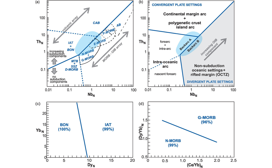
Binary classification of ophiolite-related basalts (after Saccani, 2015; with permission of Elsevier). In panels (a) and (b) the elements are normalized to the N-MORB compositions of Sun and McDonough (1989). (a) Solid line separates basalts influenced by subduction components. Central shaded area = BABB field with overlaps to IAT + BON, CAB, and the MORB–OIB array. Note progressive overlap in the MORB–OIB array from N-+ G-MORB to AB. (b) Segregation of convergent (white) and divergent (grey) tectonic settings. Within the grey field, the direction of increasing OIB component is shown by the arrow. Solid line in convergent settings separates intra-oceanic from other arc-related settings. Dashed line separates forearc and intra-arc environments from nascent forearcs. Note two types of BABB: one with subduction or crustal components (Back arc A, immature intra-oceanic or ensialic back arcs) and one lacking subduction or crustal components (Back arc B, mature intra-oceanic back arcs). Boundary coordinates in panels (a) and (b) are (0.01, 0.1), (0.01, 20), (0.5, 0.01), (0.306, 0.708), (2.2, 8.0), (100, 1000). In panels (c) and (d) the elements are normalized to the chondrite values of Sun and McDonough (1989). (c) IAT and BON may be distinguished using DyN and YbN. Boundary coordinates (9.5, 0; 7, 25). (d) N-MORB and G-MORB may be separated with CeN/YbN versus DyN/YbN. Boundary coordinates (0.4, 1.5; 2.0, 0.9). AB, Alkaline basalt; BABB, back arc basin basalt; BON, boninite; CAB, continental arc basalt; D-MORB, depleted MORB; E-MORB, enriched MORB; G-MORB, garnet MORB; IAT, island arc tholeiite; MORB, mid-ocean ridge basalt; MTB, medium-Ti basalt; N-MORB, normal MORB; OCTZ, ocean–continent transition zone; OIB, ocean island basalt; P-MORB, plume MORB; SSZ, supra-subduction zone.
5.2.2 Ti/Y–Zr/Y
The Ti/Y–Zr/Y binary diagram of Pearce and Gale (1977) discriminates between basalts from within-plate settings (continental rift and ocean island settings) and those from plate margins (island arc, continental arc and N-MORB settings) (Figure 5.2a). It utilises the enrichment in Ti (ppm) and Zr (ppm) in the source of within-plate basalts to distinguish them from plate margin basalts. Verma (2010) validated the continued use of this diagram with a data set of almost 4000 analyses (including some from E-MORB settings), which were processed using the statistical methods described in Section 5.1.4. He demonstrated that, when the E-MORB data are excluded, <11% of the data are misclassified. We conclude that this diagram is robust apart from its application to E-MORB samples which can be misclassified as within-plate basalts >40% of the time.
5.2.3 Ti/1000–V
A Ti–V discrimination diagram was first proposed by Shervais (1982). Major element (Ti) wt.% data is converted to ppm. The logic behind the diagram is that although Ti and V are adjacent members of the first transition series of the periodic table, they behave in different ways in silicate systems. The principal reason for this is that in silicate magmas V can exist in more than one oxidation state (V3+, V4+ or V5+) and yet Ti exists only as Ti4+. The redox-sensitive nature of V means that mineral–melt partition coefficients in minerals such as orthopyroxene, clinopyroxene and magnetite may vary over several orders of magnitude as a function of oxygen activity (see Section 4.2.1.3). For this reason, variations in the concentration of V relative to Ti in mafic melts reflect the oxygen activity of the magma and also any crystal fractionation processes which have taken place. These parameters can be linked to the environment of eruption and form the basis of this discrimination diagram. An added feature of the diagram is it that can be used with altered mafic compositions, for Ti and V are immobile during hydrothermal alteration and also at intermediate to high grades of metamorphism.
Vermeesch (2006a) used a training data set of 756 analyses, with SiO2 contents between 45 and 53 wt.%, from known tectonic settings and processed the data using the statistical method outlined in Section 5.1.4 to create a new Ti/1000 (ppm) versus V diagram. The new diagram is a modification of the original diagram of Shervais (1982), and the boundaries between the fields of island arc, ocean island and mid-ocean ridge basalts have been adjusted in the light of the new data set. The resulting diagram (Figure 5.2b) successfully classified 100% of the ocean island analyses, 74% of the mid-ocean ridge analyses and 70% of the island arc basalts in the test data set (n = 182). The marginal performance of island arc samples likely reflects their wide compositional variation.
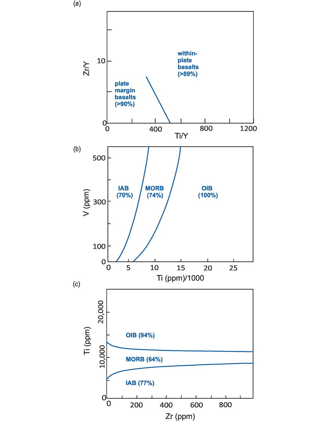
Binary classification diagrams for mafic volcanic rocks. Numbers in parentheses represent the percentage of the empirical test data set successfully classified. (a) Ti/Y versus Zr/Y (Pearce and Gale, 1977). This diagram only provides a robust statistical distinction between within-plate (rift and ocean island) and plate margin (island arc and back-arc) basalts and excludes enriched mid-ocean ridge (E-MORB) compositions (Verma, 2010). Boundary coordinates: (513, 0) and (313, 7.5). (b) Ti/1000 versus V (Shervais, 1982) with the redefined boundaries of Vermeesch (2006a; with permission from John Wiley & Sons). This diagram provides a robust statistical recognition of island arc, mid-ocean ridge and ocean island basalts. The curved boundaries of this diagram should be accurately traced or scanned. (c) Zr versus Ti (Pearce and Cann, 1973) with the redefined boundaries of Vermeesch (2006a; with permission from John Wiley & Sons). This diagram provides the robust statistical recognition of island arc and ocean island basalts, but is less reliable for MORB. The curved boundaries should be accurately traced or scanned. IAB, island arc basalt; MORB, mid-ocean ridge basalt; OIB, ocean island basalt.
5.2.4 Zr–Ti
The original Zr–Ti binary discrimination diagram of Pearce and Cann (1973) was used for basalts with a limited compositional range (20 wt.% > CaO + MgO > 12 wt.%). It also excluded alkali basalts, which were identified on the basis of their low Y/Nb ratios. The statistical reassessment of this diagram by Vermeesch (2006a) resulted in significant modifications. The original boundaries are no longer viable as there was no separation between tholeiitic and calc-alkaline basalts on the basis of their zirconium content. For this reason, the new diagram distinguishes only between island arc, ocean island, and mid-ocean ridge environments (Figure 5.2c) and correctly classifies most ocean island (94%) and island arc (77%) basalts of the test data. However, the classification of mid-ocean ridge basalts is poor (only 64% correctly classified), probably reflecting their natural variation from ‘normal’ to ‘enriched’ compositions along mid-ocean ridges.
5.2.5 Na/100–25Nb–Sr
The Na/100–25Nb–Sr triangular diagram shown in Figure 5.3a was created using robust statistical methods based on quadratic discriminant function analysis and the back-projection of the results onto triangular space (Vermeesch, 2006a). Major element (Na) wt.% data is converted to ppm. It successfully classifies all the IAB and OIB samples in the test dataset (n = 182), but is less able to correctly define MORB samples (only 58% successfully classified). The poor performance of MORB samples is probably due to Na mobility associated with seawater alteration, emphasizing the need for fresh samples.
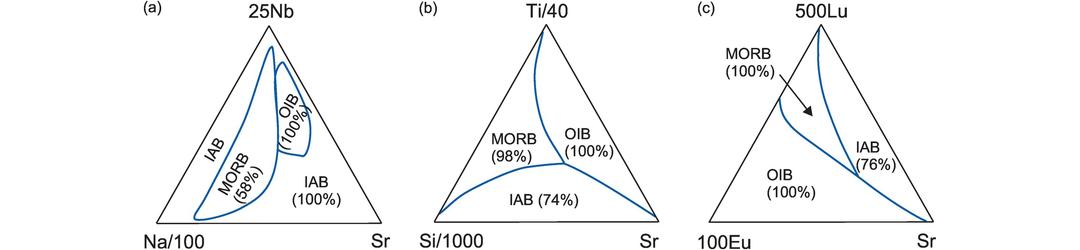
Ternary classification diagrams for mafic volcanic rocks. Numbers in parentheses represent the percentage of the empirical test data set successfully classified. Curved boundaries should be scanned. (a) Na/100–25Nb–Sr provides robust statistical classification of IAB and OIB. (b) Si/1000–Ti/40–Sr provides robust statistical classification of IAB, OIB and MORB. (c) 100Eu–500Lu–Sr provides robust statistical classification of IAB, OIB and MORB from oceanic environments.
5.2.6 Si/1000–Ti/40–Sr
The Si/1000–Ti/40–Sr triangular diagram (Figure 5.3b) was also generated through linear discriminant function analysis (Vermeesch, 2006a) and is a very successful discrimination diagram for basalts from oceanic environments (MORB, OIB and IAB). Major element (Si, Ti) wt.% data are converted to ppm. Using a test data set of 182 samples, Vermeesch (2006a) found that the diagram successfully classified 74% of the IAB samples, 98% of MORBs and all of the OIB samples.
5.2.7 100Eu–500Lu–Sr
The 100Eu–500Lu–Sr triangular diagram is based upon the differences in the REE concentrations of enriched and depleted mantle sources and can be applied to MORB, OIB and IAB. Using a test dataset of 182, Vermeesch (2006a) found that this diagram misclassifies only 24% of island arc basalt analyses (IAB) and that it correctly classifies all mid-ocean ridge basalts (MORB) and ocean island basalts (OIB) (Figure 5.3c). Given that Sr is mobile during alteration and metamorphic processes, the diagram is most applicable to pristine, unaltered basalts.
5.2.8 V–Ti/50–5Sc
Vermeesch (2006a) found that the immobile, incompatible elements V, Ti and Sc (all as ppm) are effective in distinguishing between oceanic environments when back-projected into triangular space and plotted on a V–Ti/50–5Sc diagram (Figure 5.4a). Using a test data set of 182 samples the diagram was found to work well for OIB and IAB settings (100% success), but is less effective for MORB environments, in which only 67% were classified correctly.
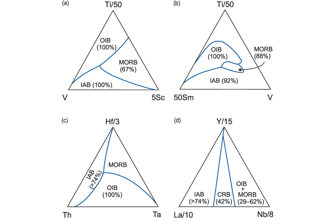
Ternary classification diagrams for mafic volcanic rocks. Numbers in parentheses represent the percentage of the empirical test data set successfully classified. The curved boundaries of this diagram need to be accurately traced or scanned. (a) V–Ti/50–5Sc (Vermeesch, 2006a; with permission from John Wiley & Sons) provides a robust statistical classification of IAB and OIB. (b) 50Sm–Ti/50–V (Vermeesch, 2006a; with permission from John Wiley & Sons) provides a robust statistical classification of IAB, OIB and MORB tectonic settings. (c) Th–Hf/3–Ta (Wood, 1980 with refined boundaries of Vermeesch, 2006a) provides a robust statistical classification of IAB and OIB; there were no MORB analyses with these elements in the test data set, but the field is well defined by the trial data. (d) La/10–Y/15–Nb/8 (Cabanis and Lecolle, 1989) provides a robust statistical classification for only IAB (island arc and back arc) tectonic settings (Verma, 2010). CRB (continental rift basalts), OIB + MORB (ocean island basalts and mid-ocean ridge basalts) are significantly misclassified.
5.2.9 50Sm–Ti/50–V
The 50Sm–Ti/50–V triangular diagram (Figure 5.4b) is based on the quadratic discriminant function analysis of immobile elements in basalts (Vermeesch, 2006a). Major element (Ti) wt.% data is converted to ppm. The classification is robust and the diagram misclassifies only 10% of the trial data. It is also successful with a test data set of 182 samples and correctly classifies OIB (100%), MORB (88%) and IAB (92%) and so is recommended for oceanic compositions.
5.2.10 Th–Hf/3–Ta
The Th–Hf/3–Ta triangular diagram (Figure 5.4c) was originally proposed by Wood (1980) and subsequently recalculated by Vermeesch (2006a). New non-linear boundaries were determined by Vermeesch (2006a) on the basis of a robust statistical analysis and the back-conversion of the data to triangular space. The new version of the diagram successfully classifies IAB (>74%) and OIB (100%) samples. There were no MORB analyses with the elements Th, Hf, Ta in the test data set, although the field was well defined by the trial data.
5.2.11 La/10–Y/15–Nb/8
The La/10–Y/15–Nb/8 triangular diagram (Figure 5.4d) for the classification of basalts was devised by Cabanis and Lecolle (1989) and more recently recalculated by Verma (2010) using a more robust statistical approach. This diagram is only reliable for island arc and back-arc (IAB) samples (<24% misclassification) and for N-MORB samples (<29% misclassification). Samples from the other tectonic environments shown in this diagram have high percentages of misclassification. Continental rift basalts (CRB) are 42% misclassified, OIB 58% and E-MORB 55%, and so this diagram should not be used for samples from these environments.
5.2.12 Major Elements
The first attempt to classify basalts from different oceanic environments using the discriminant function (DF) analysis of major element compositions was carried out by Pearce (1976). However, this work pre-dated our ability to overcome the statistical ‘closure’ problem of major element data (Section 2.2.2.1). For this reason, Vermeesch (2006a) reassessed the major element compositions of basalts using robust statistical techniques and DF analysis, and showed that it is possible to distinguish between arc, ocean-island and ocean ridge basalts. The resulting diagram is highly successful with only 7% misclassification (Figure 5.5a). The discriminant functions are based upon the oxides SiO2, Al2O3, TiO2, CaO, MgO, MnO, K2O and Na2O (note that FeO is excluded) and the definition of the DF axes is given in Appendix 5.1. Again, however, we note that while multi-element DF axes may be excellent for taxonomy and classification, they say little to illuminate petrogenetic processes.
Verma et al. (2016) proposed a DF binary diagram based upon their major element compositions to classify high-Mg rocks following the IUGS nomenclature of Le Bas (2000). The diagram was developed with a trial data set of over 900 high-Mg samples analyses, is statistically robust (<24% misclassification) and successfully classifies komatiites, meimechites, picrites and boninites.
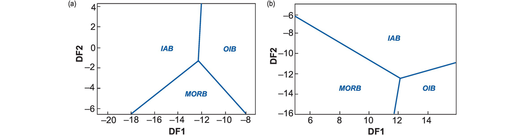
Discriminant function binary diagrams for oceanic basalts. (a) Major element oxides (without FeO) (after Pearce, 1976, and reassessed by Vermeesch, 2006a). The overall misclassification of trial data is only 7%. Boundary coordinates: central point (−12.23, −1.37), IAB–OIB (−12, 4), OIB–MORB (−8, −6.45), MORB–IAB (−18, −6.6). (b) TiO2–Zr–Y–Sr (after Butler and Woronow, 1986, and reassessed by Vermeesch, 2006a). The overall misclassification of trial data is only 8%. Boundary coordinates: central point (12.17, −12.23), IAB–OIB (15.9, −10.93), OIB–MORB (11.85, −16), MORB–IAB (5.02, −6.28). IAB, island arc basalt; MORB, mid-ocean ridge basalt; OIB, ocean island basalt. See Appendix 5.1 for discriminant function equations.
5.2.13 TiO2, Zr, Y, Sr
The TiO2–Zr–Y–Sr DF binary diagram (Figure 5.5b) was originally generated by Butler and Woronow (1986) using principal component analysis. More recently, it was statistically reassessed by Vermeesch (2006a) using the log-ratio transformation approach. This new diagram successfully classifies basalts from MORB, IAB and OIB oceanic settings with <8% misclassification, although the reader should be aware that Sr has the potential to be mobile and so the diagram is best applied to unaltered volcanic rocks. See Appendix 5.1 for the definition of the DF axes.
5.2.14 TiO2, Nb, V, Y, Zr
The TiO2–Nb–V–Y–Zr DF binary diagrams (Figure 5.6) exploit the variation between incompatible elements in ophiolitic ultramafic and mafic rocks from different tectonic settings. TiO2 is as wt.% while the other elements are in ppm. Refining the work of Pearce and Norry (1979), Verma and Agrawal (2011) statistically evaluated the chemistry of ophiolitic ultramafic and mafic rocks from four distinct settings (continental rift, ocean island, island arc and mid-ocean ridges) with a high degree of success (<10% misclassification). These diagrams are intended to be used in sequence, with the first identifying those analyses likely to be associated with the combined continental rift and ocean island field (Figure 5.6a). Once identified, these analyses are plotted on the remaining DF diagrams (Figure 5.6b–d) to minimize misclassification and better to define their most likely tectonic association. See Appendix 5.1 for the definition of the DF axes.
Discriminant function binary diagrams using Nb, V, Zr and TiO2 for ophiolitic ultramafic and mafic rocks (after Verma and Agrawal, 2011). Numbers in parentheses are the classification success rates of the empirical test data set. (a) Combines all four settings into three fields, then the other diagrams are used to improve/refine the classification. (b) Most useful for identifying island arc samples. (c) Most useful for identifying continental rift samples. (d) Most useful for identifying ocean island and mid-ocean ridge settings. Boundary coordinates in: (a) central point (0.63849, 0.87812) connects with CR+OI–IA (0.02820, 8.0), IA–MOR (8.0, −4.5532) and MOR–CR+OI (−3.2318, −8.0); (b) central point (0.883172, −0.667465) connects with IA–CR (2.27820, 8.0), CR–IA (−8.0, 1.66740) and OI–IA (1.87600, −8.0); in (c) central point (−0.016496, 0.972583) connects with IA–CR (−0.43580, 8.0), IA–MOR (8.0,-5.79920) and CR–MOR (−4.19440, −8.0); (d) central point (−0.322489, 1.040295) connects with IA–OI (−0.81840, 8.0), IA–MOR (8.0, −4.365) and OI–MOR (−3.721, −8.0). CR, continental rift;, IA, island arc; MOR, mid-ocean ridge; OI, ocean island. See Appendix 5.1 for discriminant function equations.
5.3 Elemental Discrimination Diagrams for Intermediate Volcanic Rocks
There are only a few discrimination diagrams which may be used with volcanic rocks of intermediate composition. Verma and Verma (2013) present three suites of statistically rigorous DF binary diagrams which use the following:
3. A combination of immobile major and trace elements (TiO2, MgO, P2O5, Nb, Ni, V, Y, Zr).
These diagrams may be used to distinguish those intermediate volcanic rocks which formed in island arc (IA), continental arc (CA), collisional (COL), and within-plate (combining continental rift [CR] and oceanic island [OI]) settings (Figure 5.7) and may be applied to the following rock compositions: basaltic andesite, andesite, basaltic trachyandesite, trachyandesite, tephriphonolite, phonolite and boninite. The DF analysis was based on >3600 analyses for the major element diagrams, on >1500 analyses for the immobile trace element diagrams and on >1800 analyses for the combined major and trace element diagrams. All of the analyses used outlier-free data sets from known tectonic settings.
The ‘success rate’ of each diagram is summarised in Table 5.2, and it can be seen that each of the element groups have particular strengths for identifying particular tectonic settings. The major elements provide a satisfactory indication of tectonic setting for intermediate rock compositions (Figure 5.7). However, if trace element chemistry is also available, the most confident indication for collisional settings is achieved by combining immobile major and immobile trace elements (91% success). Arc settings are best indicated by the immobile trace elements (island arc, 90% success; continental arc, 96%).
These discrimination diagrams (Figure 5.7) are intended to be used sequentially. In each case the first panel (a) successfully segregates within plate (CR + OI) and collisional (COL) settings from arc (IA + CA) settings. The remaining panels (b–d) are used to better differentiate between the different arc settings and minimize misclassification. In Figure 5.7 we present only four of the five original diagrams by Verma and Verma (2013) (shown shaded in Table 5.2) because these have the highest probability of successful classification. See Appendix 5.1 for the DF axes equations.
| Tectonic setting | A b | B b | C b | D b | E b |
|---|---|---|---|---|---|
| Major elements | |||||
| IA, island arc | 90% + 79% | 71% | 69% | 89% | – |
| CA, continental arc | 73% | 69% | – | 80% | |
| COL, collisional | 87% | – | 86% | 87% | 86% |
| CR, continental rift | 72% + 96% | 77% + 94% | – | 75% + 95% | 72% + 96% |
| OI, oceanic island | |||||
| Immobile trace elements | |||||
| IA, island arc | 91% + 90% | 76% | 73% | 90% | – |
| CA, continental arc | 66% | 65% | – | 96% | |
| COL, collisional | 81% | – | 84% | 85% | 81% |
| CR, continental rift | 74% + 100% | 81% + 100% | – | 75% + 100% | 74% + 94% |
| OI, oceanic island | |||||
| Immobile majors + traces | |||||
| IA, island arc | 86% + 89% | 70% | 63% | 86% | – |
| CA, continental arc | 82% | 76% | – | 95% | |
| COL, collisional | 90% | – | 93% | 90% | 91% |
| CR, continental rift | 73% + 100% | 79% + 100% | – | 74% + 99% | 73% + 99% |
| OI, oceanic island |
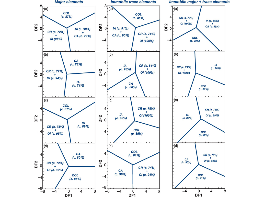
Major element discriminant function binary diagrams for intermediate rocks (after Verma and Verma, 2013). Numbers in parentheses represent the percentages of successfully classified test data. All diagrams combine five tectonic settings into three fields (a panels) and use subsequent diagrams (b–d) to separate the two arc environments. Major elements: (a) Initial groupings. Central point (−0.67554, 0.27663), CR + OI–COL (−8.0, 4.73569), COL–IA + CA (8.0, 5.53331), IA + CA–CR + OI (0.42744, −8.0). (b) Shows the separation of CA from IA. Central point (−0.63205, 0.08764), CR + OI–CA (−2.73408, 8.0), CA–IA (8.0, 0.76690), IA–CR + OI (−1.50230, −8.0). (c) Most useful for identifying continental arc rocks. Central point (−0.44102, 0.17933), CR + OI–COL (−8.0, 4.24657), COL–IA (8.0, 6.27226), IA–CR + OI (0.66776, −8.0). (d) Most useful for identifying continental rift, island arc and collisional settings. Central point (−0.033967, −0.10997), CR + OI–CA (−3.42497, 8.0), CA–COL (8.0, −0.16286), COL–CR + OI (−4.17272, −8.0). Immobile trace elements: (a) Initial groupings. Central point (0.64148, 0.34301), IA + CA–COL (−6.91145, 8.0), COL–CR + OI (8.0, 3.04640), CR + OI–IA + CA (−0.69292, −8.0). (b) Shows the separation of CA and IA. Central point (0.58959, 0.68699), CA–IA (−8.0, −5.45793), IA–CR + OI (0.87619, 8.0), CR + OI–CA (3.67939, −8.0). (c) Most useful for identifying IA and COL. Central point (0.37157, −0.26385), IA–CR + OI (−0.87235, 8.0), CR + OI–COL (8.0, −2.82217), COL–IA (−6.10890, −8.0). (d) Most useful for identifying CA. Central point (−0.15459, 0.29462), CA–COL (−8.0, 5.41425), COL–CR + OI (8.0, 4.74335), CR + OI–CA (−0.10284, −8.0). Immobile majors + trace elements: (a) Initial groupings. Central point (−0.82858, 0.29965), CR + OI–IA + CA (0.92190, 8.0), IA + CA–COL (6.39297, −8.0), COL–CR + OI (−8.0, −4.20284). (b) Provides an initial separation of IA and CA. Central point (−0.95018, 0.45941), CR + OI–IA (−1.24490, 8.0), IA–CA (8.0, −3.76290), CA–CR + OI (−3.41007, −8.0). (c) Most useful for identifying IA. Central point (0.62149, 0.34939), IA–CR + OI (−0.87616, 8.0), CR + OI–COL (8.0, −4.51524), COL–IA (−6.61289, −8.0). (d) Most useful for identifying CA and COL. Central point (−0.028516, 0.35743), CA–CR + OI (−1.16430, 8.0), CR + OI–COL (8.0, −3.84452, COL–CA (−7.33632, −8.0). CA, continental arc; CR, continental rift; COL, collisional; IA, island arc; OI, oceanic island. See Appendix 5.1 for discriminant function equations.
5.4 Elemental Discrimination Diagrams for Acid Plutonic Rocks
The first systematic study in which granite geochemistry was related to tectonic setting was by Pearce et al. (1984). In this study the term ‘granite’ was defined very loosely as ‘any plutonic rock containing more than 5 per cent of modal quartz’. Using suite of 600 selected granites, the authors determined that the elements Y, Yb, Rb, Ba, K, Nb, Ta, Ce, Sm, Zr and Hf most effectively discriminated between ocean ridge (ORG), volcanic-arc (VAG), within-plate (WPG) and syn-collisional (S-COLG) granite types. Verma et al. (2012) reassessed these data using modern statistical methods and concluded that ORGs cannot be classified using this approach (although the number of ORG samples in the original data set was very low, n = 5).
5.4.1 The Yb–Ta and Y–Nb Discrimination Diagrams
In their reassessment of trace element-based discrimination diagrams for granites, Verma et al. (2012) argued that the Yb–Ta and Y–Nb binary diagrams originally proposed by Pearce et al. (1984) have limited functionality. However, if ORG samples can be excluded from the data set on the basis of their field setting, then these diagrams can be used to distinguish between WPG, VAG and S-COLG. For example, the Yb–Ta diagram successfully differentiates between WPG (no misclassification), VAG (11% misclassification), and S-COLG (~25% misclassification) (Figure 5.8a), and the Y–Nb diagram successfully separates WPG (~18% misclassification) from the combined field of VAG + S-COLG (~4% misclassification) (Figure 5.8b).
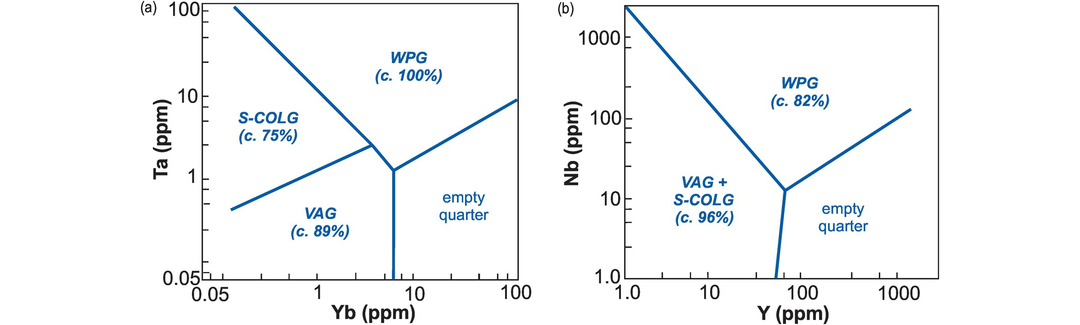
Trace element binary diagrams for granites (modified from Pearce et al., 1984). Numbers in parentheses represent the percentages of successfully classified test data (Verma et al., 2013). (a) Yb/Ta successfully distinguishes between VAG, S-COLG and WPG. Boundary coordinates: VAG–S-COLG (0.1, 0.35; 3, 2); S-COLG–WPG (0.1, 100; 3, 2), VAG–WPG (3, 2; 5, 1); WPG–empty (5, 1; 100, 7), empty–VAG (5, 0.05; 5, 1). (b) Y/Nb successfully separates VAG + S-COLG from WPG. Central point (50, 10), VAG + S-COLG–WPG (1, 2000), WPG–empty (1000, 100), empty–VAG + S-COLG (40, 1). S-COLG, syn-collisional; VAG, volcanic-arc; WPG, within-plate.
5.4.2 Major Element Diagrams
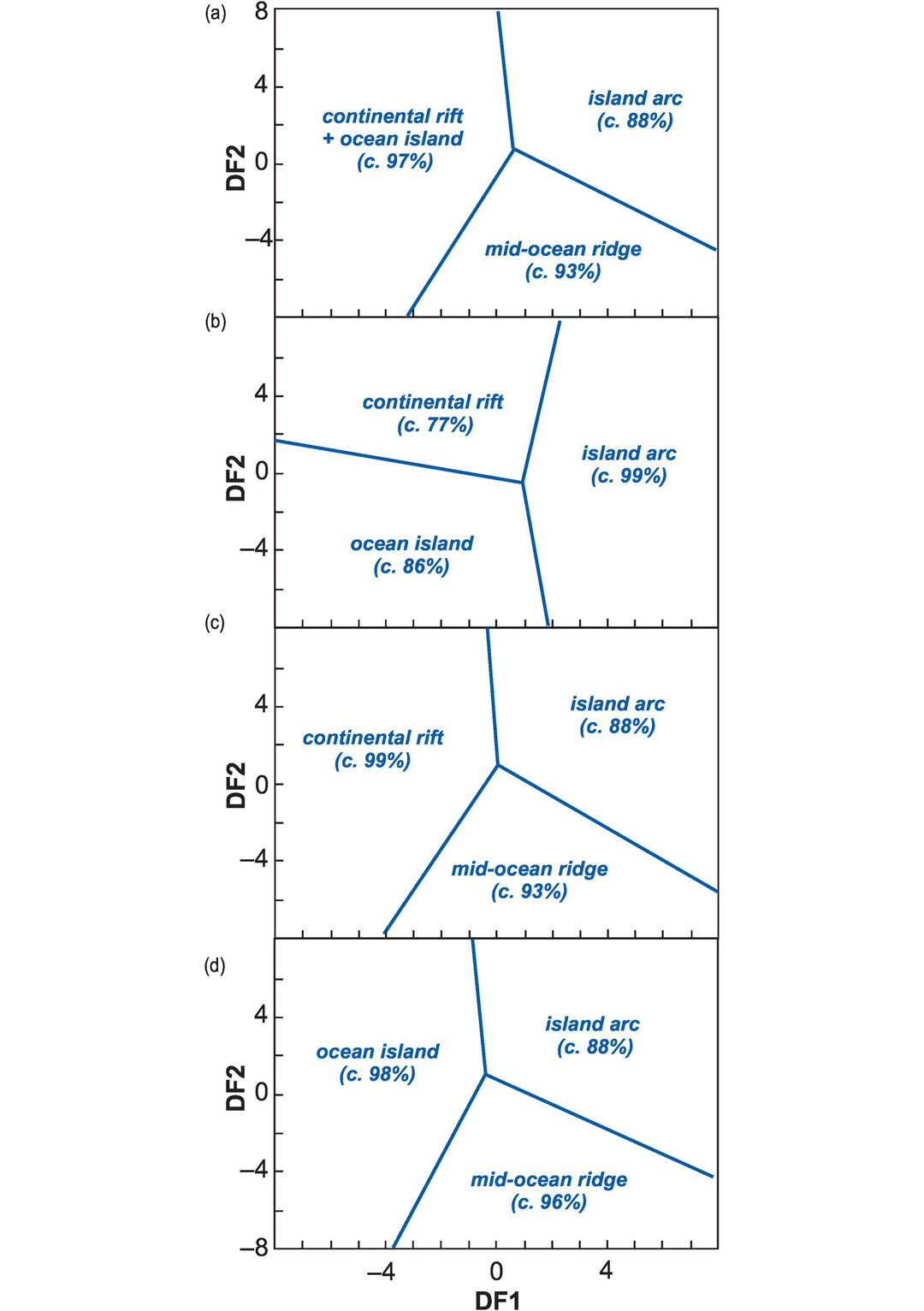
A series of DF binary diagrams (Figure 5.9) based upon granite major element chemistry was proposed by Verma et al. (2012). The DF diagrams were generated using robust statistical methods (see Section 5.1.2) and based upon a trial data set of >1000 outlier-free analyses, all with SiO2 > 63 wt.% and from known tectonic settings. The test data set contained 100 analyses. This suite of diagrams distinguishes between granitoids from island arc (IA), continental arc (CA), continental rift (CR), and continental collisional (COL) settings. As usual for DF analysis, the first diagram presents all the data, in this case by combining the two arc settings (IA + CA). The subsequent diagrams are then used to better segregate the two arc settings and minimize misclassification (generally better than 16%). Here we have selected the three most successful diagrams of the original five diagrams presented by Verma et al. (2012). The DF equations include all the major element oxides and are given in Appendix 5.1.
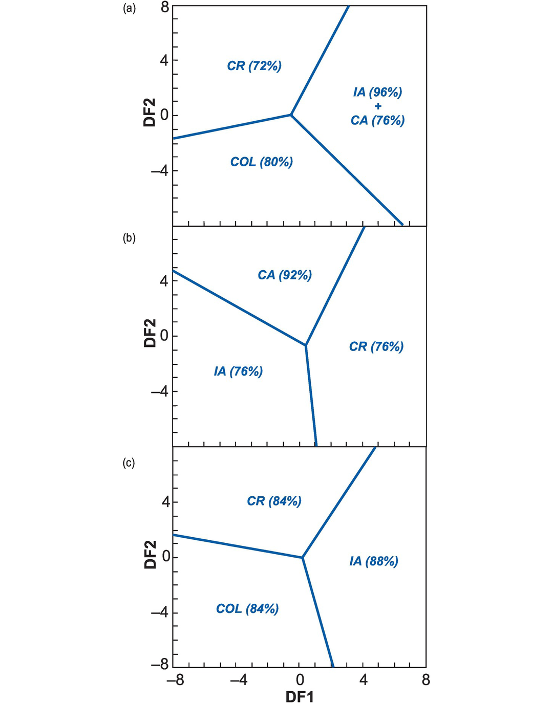
Major element discriminant function binary diagrams for acid rocks from island arc, continental arc, continental rift and syn-collisional tectonic settings (after Verma et al., 2012). ‘Acid rocks’ are those with >63 wt.% SiO2 (anhydrous, Fe oxidation state of Middlemost, 1989). Numbers in parentheses represent the classification success rates of the empirical training data. (a) The initial groupings. Central point (−0.52237, 0.105108), CR–IA + CA (3.0914, 8.00), IA + CA–COL (6.5177, −8.00), COL–CR (−8.00, −1.6511). (b) This figure effectively identifies CA. Central point (0.41929, −0.66705), CA–CR (4.1608, 8.00), CR–IA (1.0939, −8.00), IA–CA (−8.00, 4.7147). (c) This panel effectively separates CR, AI and COL. Central point (0.20518, −0.01689), CR–IA (4.7956, 8.00), IA–COL (2.1584, −8.00), COL–CR (−8.00, 1.61186). See Appendix 5.1 for discriminant function equations.
5.4.3 Some Words of Caution
There are a number of pitfalls that may be encountered when using discrimination diagrams with granitic lithologies. These are identified below.
1. Increasingly, it is becoming clear that the chemical composition of granitic rocks does not always represent the composition of a simple melt but is instead a mix of crystals and melt (Collins et al., 2020). For this reason, discrimination diagrams for granitic rocks should be used with great care.
2. Granitic melt compositions are often modified by the effects of crystal fractionation and, late in their crystallisation, by their interaction with hydrothermal fluids. This will influence those discrimination diagrams which are based upon major element chemistry such as the DF diagrams of Verma et al. (2012).
3. Finally, it is necessary to repeat the words of caution given earlier about the general use of discriminant function diagrams. DF diagrams can work quite well if their principal purpose is to classify rocks and assign rock suites to their former tectonic setting. Nevertheless, the discriminant functions themselves are petrologically opaque and are unable to help us evaluate geochemical processes.
5.5 Discrimination Diagrams for Clastic Sediments
Sedimentary basins form through the extensional, compressional or transcurrent motion of the Earth’s tectonic plates. A large number of different types of basin are associated with each of these settings and are summarised in Box 5.2. Sediment may inherit a geochemical signature from its tectonic environment in two separate ways. First, different tectonic environments may have distinctive provenance characteristics which can be transposed into the sedimentary record. Second, some tectonic environments may be characterised by distinctive sedimentary processes. In both cases the geochemical signature is most likely to be seen in immature sediments which contain lithic fragments and so directly reflect the composition of their source. From this information the provenance may be identified and from the provenance the tectonic setting may often be inferred.
Divergent plate motion
Continental rift
Oceanic rift on a ridge
Proto-oceanic rift
Cratonic (intracontinental) basins
Rift-sag (failed rift) basins
Passive margin basins
Active oceanic (abyssal) basins
Convergent plate motion
Oceanic islands, aseismic ridges, plateaus
Oceanic trench
Fore-arc basins
Back-arc basins
Intramontaine/intra-arc basins
Pro-(peripheral) foreland basins
Retro-foreland basins
Thrust sheet-top (piggyback) basins
Transcurrent plate motion
Transtensional (pull-apart) basins
Transpressive basins
Transrotational basins
Since the 1980s, when many of the discrimination diagrams for clastic sediments were first developed, it has become apparent that there are a number of factors which can distort the geochemical signature of sediments such that it will not reflect the true tectonic setting of deposition. These factors include the heterogeneities which are associated with the initial source region, the weathering of the source rocks, the differences in mineral size/shape/density created through physical sorting and the mineralogical alteration that takes place during hydrological transport and diagenesis.
Some early studies claimed to successfully define the tectonic setting of a sedimentary basin using geochemical data from clastic sediments (e.g., Bhatia, 1983; Roser and Korsch, 1986), although the more recent reassessment of these diagrams using robust statistical techniques has found that the majority (>70%) are now known to be unable to discriminate between active and passive margin settings (Table 5.1). Consequently, the sediment which most faithfully records its original tectonic setting via its geochemistry must be locally derived, proximal to its source and juvenile in character, and even then the results must be critically evaluated. Sediment that has been recycled or derived from mixed sources is not easily interpreted, although Totten et al. (2000) outline some approaches that may be used to extract information about provenance and tectonic setting from more mature sediments. There are also some instances when DF analysis may successfully distinguish between clastic sediments formed in arc, rift and collisional tectonic settings (Section 5.5.1).
5.5.1 A Discrimination Diagram for Sand-Sized Clastic Sediment
The DF binary diagram of Verma and Armstrong-Altrin (2013) (Figure 5.10) discriminates between arc, rift and collisional settings in sand-sized clastic sediment (Table 5.1). The diagram is based on ten major element oxides (SiO2, Al2O3, CaO, Na2O, K2O, P2O5, TiO2, MnO, MgO, FeOT) and its effectiveness is optimised when clastic sediments are divided into high-silica (SiO2 = 63–95 wt.%) and low-silica (SiO2 = 35–63 wt.%) groups. The field boundaries were determined using a trial dataset of >2200 analyses; the DFs are given in Appendix 5.1. Both diagrams successfully differentiate between arc settings in which there is active volcanism, extensional rift settings and sediments formed in a collisional, compressional setting (<25% misclassification). These authors also demonstrate that the chemical changes caused by weathering, recycling and diagenesis are unlikely to significantly affect the results of major element DF analysis.
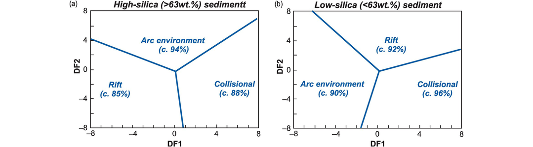
Major element discriminant function binary diagrams for classification of siliciclastic sediment from arc, rift and syn-collisional tectonic settings (after Verma and Armstrong-Altrin, 2013). Numbers in parentheses represent the classification success rates of the empirical test dataset. (a) High-silica sediment. Central point (0.051, −0.220), Arc–Col (8, 7.090), Col– Rift (0.794, −8), Rift–Arc (−8, 4.153). (b) Low-silica sediment. Central point (0.180, −0.178), Arc–Rift (−6.226, 8), Rift–Col (8, 2.822), Col–Arc (−1.629, −8). See Appendix 5.1 for discriminant function equations.
5.5.2 Discrimination Diagrams for Fine-Grained Clastic Sediment
The use of shale or mudstone chemistry to determine tectonic setting is based on the assumption that fine-grained rocks efficiently homogenise source materials and therefore can be used to determine the tectonic setting in which the rock was deposited (Condie et al., 1991). Fine-grained sediment chemistry is often normalized to the composition of the upper continental crust (UCC; Rudnick and Gao, 2014) or to various shale composites such as the North American shale composite (NASC; McLennan, 1989) or the post-Archaean Australian shale (PAAS; Pourmand et al., 2012) (see Section 4.3.2.4 and Table 4.8) in order to illustrate the degree to which the composition of the sediment is different from the average composition of the continental crust.
A useful application of a NASC-normalised multi-element diagram is given by Totten et al. (2000). These workers compare normalized average compositions for the Stanley shale from the Ouachita Mountains to the normalized average values of passive and combined active and continental arc margins of Floyd et al. (1991). They concluded that the Stanley shale was derived from a mixed provenance which included felsic and mafic sources. The values for the normalized average values of passive and combined active and continental arc margins are shown in Figure 5.11. Average passive margin sediments are characterised by negative anomalies for the elements Sr, Ta and Nb and positive anomalies for the elements U, Cs, Ti, Hf and Zr, whereas the average arc margin sediments are characterised by negative Ta and Nb anomalies and positive Ba, Cr, Ni, Ti and Sc.
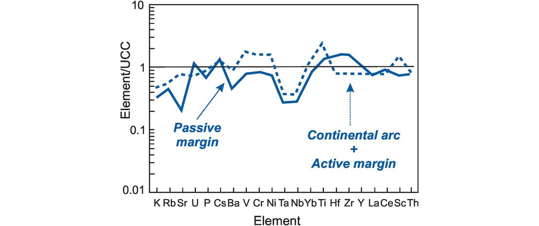
Multi-element discrimination diagram for shale (after Floyd et al., 1991) showing the normalized average values for passive margins (solid line) and the normalized combined average for continental arc and active margins (dashed line). The sedimentary compositions are normalized to the upper continental crust values of Taylor and McLennan (1985).
5.5.3 Provenance Studies
The use of trace elements as indicators of provenance in fine-grained sediments has been discussed by Cullers et al. (1988), Condie and Wronkiewicz (1990), McLennan and Taylor (1991) and Totten et al. (2000). These authors have exploited the geochemical differences between elements in fine-grained sediments such as Th and La (indicative of a felsic igneous source) and Sc and Cr (indicative of a mafic source), and have used plots such as Th/Sc versus Sc and Cr/Th versus Sc/Th as indicators of contrasting felsic and mafic provenance in shales. Floyd et al. (1989) quantified such mixing processes using the general mixing equation of Langmuir et al. (1978) discussed in Section 4.8.2.5, and Tang et al. (2016) sought to identify the proportion of mafic components in sediments using Ni/Co and Cr/Zn ratios. This work was based upon the argument that Ni and Cr are more compatible in early fractionating phases in mafic rocks than are Co and Zn and that these elements are normally insoluble during chemical weathering, hence the ratios Ni/Co and Cr/Zn are a useful indicator of the mafic contribution to fine-grained sediments. Their study also suggested that over Earth history the mafic component in fine-grained sediments has decreased with time. Totten et al. (2000) used Th/Sc ratios to characterise mafic and felsic sources, as illustrated in Figure 5.12. However, we recommend that diagrams using common denominator ratio pairs such as Th/Sc versus La/Sc should be used with care because of the possible effects of spurious self-correlation.

Immobile element discrimination diagram for shales. The incompatible element Th is enriched in silicic rocks, whereas the compatible element Sc is enriched in mafic rocks. Thus Th/Sc near unity suggests upper continental crustal derivation, whereas Th/Sc near 0.6 suggests a dominant mafic component.
5.6 Tectonic Controls on Magmatic and Sedimentary Geochemistry
The underlying tectonic controls on the chemistry of magmatic and sedimentary rocks is an issue which is much wider than that of discrimination diagrams (see Condie, 2015; Li et al., 2015, for discussion), and is a major focus of much of modern geochemistry. In recent decades, our understanding of tectonic processes and their influence on trace element and isotope geochemistry has grown exponentially. Alongside this we have also learned something of the inherent complexity of both tectonic systems and of geochemical processes. For this reason, a naive ‘cookbook’ approach to the identification of former tectonic environments by means of geochemical fingerprinting is unproductive, and likely to bypass the fundamental processes which are operating in those environments. Consider a few examples:
1. A basaltic melt which assimilates continental crust. During transit through the crust, the basaltic melt assimilates continental crustal material. In this case, the geochemical signature of the basalt may be predominantly inherited from the crustal source and not reflect its tectonic setting.
2. Secular variation in Earth history. The composition of the mantle has likely changed with time given the secular variation of the Earth’s temperature, the chemical differentiation of its mantle composition and the recycling of tectonic plates over 4.6 Ga. Clearly, this variation imposes limits on the projection of modern geochemical signatures through time.
3. The derivation of tectonic information from fine-grained sediment. Fine-grained clastic sediments are often far removed from their source(s) and compositionally altered to clay, making it difficult to extract meaningful information from them regarding the tectonic setting from which they were derived.
Given such complexities, it is important to progress beyond simplistic classification in order to understand the petrological processes involved in, and thereby the petrogenetic links between, geochemistry and tectonic setting. There are two other important factors that we have sought to emphasise in this chapter. First, it is necessary to perform a rigorous statistical evaluation of any ternary, bivariate or multivariate diagram. Only after trial testing with large data sets from known settings and after dealing with the problems of closure and spurious self-correlation should a tectonic discrimination diagram be used by the geochemical community. Even then, discrimination diagrams should not be regarded as a proof; rather, they are a guide to a testable hypothesis which may be validated through a more comprehensive geological and geochemical evaluation. Second, in our view the primary function of geochemical data is to reveal geochemical, and thereby geological, processes. These in turn can make apparent petrological processes which can (sometimes) help to identify the tectonic environment in which those processes have taken place. It is in this spirit that we must approach the use of tectonic discrimination diagrams.