6.1 Introduction
Radiogenic isotopes are used in geochemistry in two principal ways: (i) to determine the age of rocks and minerals and (ii) to identify geological processes and sources. The former application is geochronology, while the latter is known as isotope geology or isotope geochemistry. There are some excellent texts which deal with these disciplines (e.g., Rink and Thompson, 2015; White, 2015; Reiners et al., 2018) and the reader is referred to these for more detailed treatments of the topics introduced here.
In the first part of this chapter the main principles of geochronology are briefly described and the interpretation of geochronological results reviewed. The second half of the chapter describes the use of radiogenic isotopes in petrogenesis, an exciting and rapidly evolving field. The use of radiogenic isotopes as tracers of petrogenetic processes has allowed geochemists to sample the deep interior of the Earth, previously the sole domain of geophysicists. The results of such studies have led to important geochemical constraints on the nature of the continental crust and the Earth’s mantle, which can be combined with our physical knowledge of these domains to help provide a unified chemical-physical model of the deep Earth.
6.2 Radiogenic Isotopes in Geochronology
The foundations of modern geochronology were laid at the turn of the century in the work of Rutherford and Soddy (1903) on natural radioactivity. They showed that the process of radioactive decay is exponential and independent of chemical or physical conditions. Thus, rates of radioactive decay may be used for measuring geological time. The isotopic systems used in age calculations are listed in Table 6.1 and Box 6.1. In this section we discuss two of the most common techniques used in geochronological calculations: isochron diagrams and model age calculations. This is followed by a discussion of the significance of the calculated ages.
| Technique | Decay scheme | Decay constant λ (yr−1) | Reference | Isochron plot | |
|---|---|---|---|---|---|
| x-axis | y-axis | ||||
| Rb–Sr | 87Rb → 87Sr + β | 1.42 × 10⁻¹¹ | 1a | 87Rb/86Sr | 87Sr/86Sr |
| Sm–Nd | 147Sm → 143Nd + He | 6.54 × 10⁻¹² | 2 | 147Sm/143Nd | 143Nd/143Nd |
| Lu–Hf | 176Lu → 176Hf + β | 1.867 × 10⁻¹¹ | 3b | 176Lu/177Hf | 176Hf/177Hf |
| Re–Osc | 187Re → 187Os + β | 1.666 × 10⁻¹¹ | 4 | 187Re/188Os | 187Os/188Os |
| 187Re (ppb) | 187Os (ppb) | ||||
| K–Ar | 40K → 40Ar − β | 0.581 × 10⁻¹⁰ | 1d | 40K/36Ar | 40Ar/36Ar |
| 39Ar/36Ar | 40Ar/36Ar | ||||
| K–Cac | 40K → 40Ca + β | 4.962 × 10⁻¹⁰ | 1, 5 | 40K/42Ca | 40Ca/42Ca |
| K total | 5.543 × 10⁻¹⁰ | 1 | |||
| La–Cec | 138La → 138Ce + β | 2.37 × 10⁻¹² | 6 | 138La/136Ce | 138Ce/136Ce |
| La–Bac | 138La → 138Ba − β | 4.44 × 10⁻¹² | 7 | 138La/137Ba | 138Ba/137Ba |
a Officially accepted value today, but other values exist and may be in use (1.393 × 10⁻¹¹; Nebel et al., 2011). Older data use λ87Rb = 1.39 ×10⁻¹¹ and can be recalculated for the modern decay constant using a correction factor (e.g., 1.39/1.42).
b Older data use λ176Lu = 1.94 × 10⁻¹² (DePaolo, 1988) or 1.96 × 10⁻¹² (Patchett and Tatsumoto, 1980).
c Specialist techniques carried out in only a few laboratories.
References: 1, Steiger and Jager (1977); 2, Lugmair and Marti (1978); 3, Söderlund et al. (2004); 4, Smoliar et al. (1996); 5, Marshall and DePaolo (1982); 6, Tanimizu (2000); 7, Sato and Hirose (1981).
(a) Decay constants (Steiger and Jager, 1977)
238U » 206Pb 1.55125 × 10⁻¹⁰ yr−1 (λ1)
235U » 207Pb 9.8485 × 10⁻¹⁰ yr−1 (λ2)
232Th » 208Pb 4.9475 × 10⁻¹¹ yr−1 (λ3)
(b) Isotope ratios of primeval lead (represented by Canyon Diablo troilite of Tatsumoto et al., 1973)
(206Pb/ 204Pb) = 9.307
(207Pb/ 204Pb) = 10.294
(208Pb/ 204Pb) = 29.476
(c) Age of the Earth derived from the meteoritic isochron (Tatsumoto et al., 1973; Tilton, 1973)
207Pb/ 204Pb versus 206Pb/ 204Pb yields an isochron with a slope = 0.626208 and an age for the Earth of 4.57 Ga.
(d) Present day ratio 238U/ 235U = 137.88
(e) Symbols used in U–Th–Pb isotope geochemistry
μ = 238U/204Pb, κ = 232Th/238U
(f) Ratios used for plotting the U–Pb concordia curve
| Age (Ga) | 206Pb/238U | 207Pb/235U |
|---|---|---|
| 0.0 | 0.00000 | 0.00000 |
| 0.4 | 0.06402 | 0.48281 |
| 1.0 | 0.16780 | 1.67741 |
| 1.4 | 0.24256 | 2.97009 |
| 1.8 | 0.32210 | 4.88690 |
| 2.2 | 0.40674 | 7.72917 |
| 2.6 | 0.49679 | 11.94371 |
| 3.0 | 0.59261 | 18.19308 |
| 3.4 | 0.69456 | 27.45973 |
| 3.6 | 0.74796 | 33.65562 |
| 3.8 | 0.80304 | 41.20041 |
| 4.0 | 0.85986 | 50.38776 |
| 4.2 | 0.91846 | 61.57526 |
| 4.4 | 0.97892 | 75.19836 |
| 4.6 | 1.04128 | 91.78732 |
6.2.1 Isochron Calculations
An isochron diagram is a bivariate plot of measured parent–daughter isotope ratios for a suite of cogenetic samples or for a mineral suite from a single sample. When the sample suite defines a linear array, this is said to be an isochron, and the slope of the line is proportional to the age of the sample suite. Consider, for example, the Rb–Sr system where the total number of 87Sr atoms in a rock which has been a closed system for t years is given by the equation:
87Srm is the total number of atoms of 87Sr present today, 87Sri is the number of atoms of 87Sr initially present when the sample first formed, 87Rbm is the number of atoms of 87Rb present (measured) today, and λ (lambda) is the radioactive decay constant (Table 6.1). The precise measurement of absolute isotope concentrations is difficult, so instead isotope ratios are normally determined. An isotope not involved in the radioactive decay scheme is used as the denominator. In the case of the Rb–Sr isotope system this isotope is 86Sr and Eq. 6.1 is rewritten as:
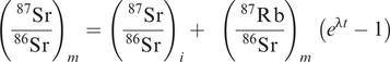
The ratios (87Sr/86Sr)m and (87Rb/86Sr)m are measured by mass spectrometry, leaving the initial ratio (87Sr/86Sr)i and the age of the rock (t) as unknowns. Since Eq. 6.2 is the equation of a straight line, the age and intercept can be calculated from a plot of measured (87Sr/86Sr)m and (87Rb/86Sr)m for a suite of cogenetic samples. This methodology is illustrated in Figure 6.1. The age is calculated from the slope of the line using the equation
where t is the age and λ is the decay constant. Time is measured from the present and is expressed as either Ma (106 years) or Ga (109 years). The intercept on the (87Sr/86Sr) axis is equal to the initial ratio (87Sr/86Sr)i, a parameter of considerable petrogenetic importance and discussed more fully later in this chapter.
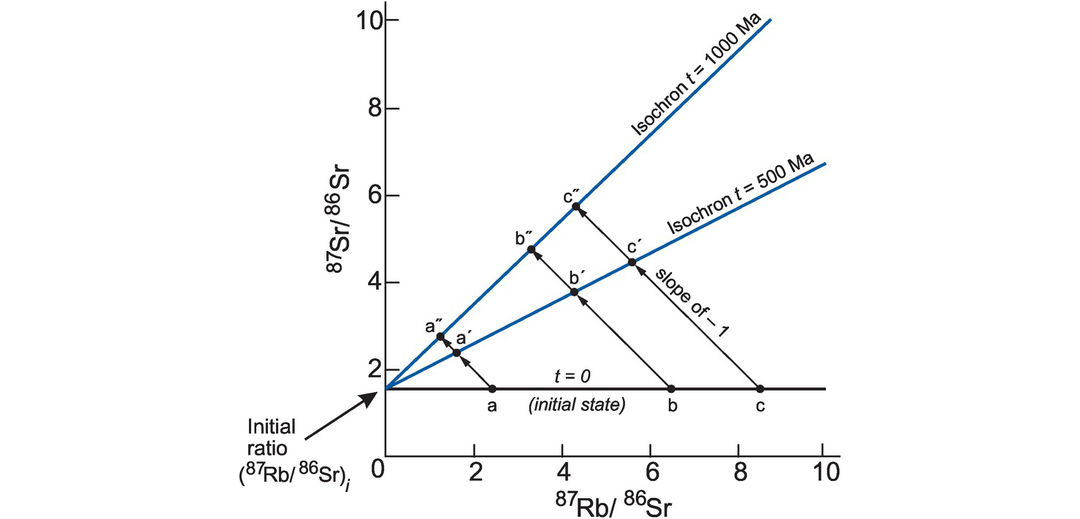
Schematic isochron diagram. A suite of igneous rocks (a–c) form at t = 0 from the same batch of magma which subsequently differentiated. They evolve over 500 Ma and 1000 Ma. At t = 0 each member of the rock suite has the same initial ratio (87Sr/86Sr)i but because the magma suite is chemically differentiated, each rock has a different concentration of Rb and Sr, and therefore a different 87Rb/86Sr ratio. Each sample plots as a separate point on the 87Rb/86Sr versus 87Sr/86Sr isochron diagram. From t = 0 to t = 500 Ma or t = 1000 Ma, individual samples evolve along a straight line with a slope of −1 (e.g., a–a′–a′′) reflecting the decay of a single atom of 87Rb to a single atom of 87Sr. In practise the resulting change in 87Sr/86Sr is small and the vertical scale is normally exaggerated so the path taken by these points will be closer to a vertical line. The amount of 87Sr produced in a given sample is proportional to the amount of 87Rb present. The slope of each isochron (t = 500 Ma, t = 1000 Ma) is proportional to the age of the sample suite. The intercept on 87Sr/86Sr is the initial ratio.
Thus, an isochron calculation requires a suite of cogenetic samples formed from the same parental material – this may be a suite of whole rock samples from a single pluton or a suite of different minerals from a single sample. The isochron calculation assumes that there has been no exchange of parent–daughter isotopes other than through radioactive decay. An example of a Sm–Nd isochron derived from a suite of related volcanic rocks using the data in Table 6.2 is shown in Figure 6.2.
| Sample | Rock type | 147Sm/144Ndb | 143Nd/144Nd |
|---|---|---|---|
| (± 2σ error) | |||
| HSS-74 | Sodic porphyry | 0.1030 | 0.510487 ± 36 |
| HSS-161 | Acid tuff | 0.1054 | 0.510570 ± 32 |
| HSS-52B | Felsic pillow lava | 0.1653 | 0.511950 ± 22 |
| HSS-56 | Basaltic lava | 0.2040 | 0.512875 ± 32 |
| R-14 | Basaltic komatiite | 0.1888 | 0.512504 ± 34 |
| HSS-32 | Basaltic komatiite | 0.1649 | 0.511957 ± 22 |
| HSS-88A | Peridotitic komatiite | 0.1792 | 0.512292 ± 34 |
| HSS-92 | Peridotitic komatiite | 0.1858 | 0.512439 ± 34 |
| HSS-95 | Peridotitic komatiite | 0.1902 | 0.512541 ± 28 |
| HSS-523 | Peridotitic komatiite | 0.1701 | 0.512084 ± 20 |
a Hamilton et al. (1979b); data used to construct Figure 6.2.
b 147Sm/144Nd determined to a precision of 0.2% at the 2σ level.
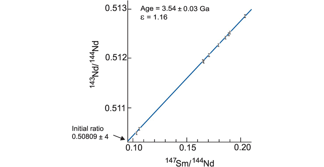
A Sm–Nd isochron. An isochron plot of 147Sm/144Nd and 143Nd/144Nd for volcanic rocks from the Onverwacht group, South Africa (after Hamilton et al. (1979b)). The data are given in Table 6.2. Error bars for 143Nd/144Nd are 2σ (errors on 147Sm/144Nd are too small to show). The slope of the best fit line is proportional to the age or the suite (3.54 ± 0.03 G(a); the intercept of this line on the 143Nd/144Nd axis where 147Sm/144Nd = 0 is the initial 143Nd/144Nd ratio (0.50809 ± 0.00004). The εNd value (+1.16) is a measure of the difference between the initial ratio and a chondritic model for the Earth’s mantle at 3.54 Ga expressed in parts per 10,000 (see Section 6.3.4 and Box 6.2). The positive value for εNd indicates that the volcanic rocks were derived from a (slightly) depleted mantle source at 3.54 Ga, although there are large errors on this estimate.
6.2.1.1 Pb Isotope Isochrons
A Pb–Pb whole rock isochron is constructed by plotting the isotope ratios 206Pb/204Pb on the x-axis and 207Pb/204Pb on the y-axis. However, the interpretation of a linear array on this diagram is more complicated than for the Rb–Sr system because 206Pb and 207Pb are the products of separate radioactive decay schemes with different rates of decay (Box 6.1). In this case the isochron equation and must be solved iteratively (see Harmer and Eglington, 1987); see Section 6.2.5.3.
6.2.1.2 Fitting an Isochron
A simple but approximate method to fit an isochron is to draw a best-fit straight line by eye through the plotted points. Provided a suitable scale is chosen, both the slope of the line and the intercept can be determined with reasonable accuracy and these may be used to make preliminary estimates of the age and initial ratio. Precise results are obtained from statistical line-fitting procedures which estimate the slope and intercept of the isochron. These normally use a version of weighted least squares regression (see Section 2.5) and standard equations can be found in Excel, IsoplotR (Vermeesch, 2018b), and other statistical packages.
An important aspect of isochron regression is the realistic estimate of the uncertainty associated with the age and initial ratios. A measure of the ‘goodness of fit’ of an isochron is the mean squares of weighted deviates (MSWD). This is a measure of the fit of the line to the data within the limits of analytical error. Ideally, an isochron should have a MSWD of ≤ 1; anything greater than this implies that the scatter in the data points cannot be explained solely by experimental error. However, Brooks et al. (1972) suggest that this value be restricted to isochrons involving infinitely large numbers of samples, whereas for more typical datasets higher values up to ~2.5 may be acceptable.
6.2.1.3 Errorchrons
The origin of the scatter on an isochron is one of the most important interpretive aspects of geochronology. If the scatter results in a MSWD of ≤2.5, it is deemed analytical. If the MSWD is >2.5, it is geological. Brooks et al. (1972) proposed the term ‘errorchron’ for the situation where a straight line cannot be fit to a suite of samples within the limits of analytical error. An errorchron by definition implies that the scatter of the data is a consequence of geological error and indicates that one or more of the initial assumptions of the isochron has not been fulfilled, that is, that the samples are not cogenetic or that there has been subsequent parent–daughter isotopic exchange.
6.2.1.4 The Geochron
The geochron represents an isochron drawn at t = 0 and uses the composition of the appropriate isotope ratio at the time the Earth formed, that is, the Earth’s primordial isotopic composition. In principle, a geochron can be defined for any isotopic system, although in practice it is most commonly used in the interpretation of lead isotopes and is used as a reference line in some lead isotope studies. The lead isotope geochron (constructed as in Section 6.2.1.1) is calculated using the initial values for the Earth given in Box 6.1(b) for ages between 4.4 and 4.6 Ga. Its precise position is a function of the presumed age of the Earth, and so although a geochron represents a zero age isochron, the age of the Earth used in its computation (say, 4.57 Ga) must also be specified.
6.2.2 Model Ages
A model age is a measure of the length of time a sample has been separated from the mantle from which it was originally derived. Model ages are most commonly quoted for the Sm–Nd and Lu–Hf systems and can be calculated for an individual rock from a single pair of parent–daughter isotopic ratios. They must, however, be interpreted with care as the basis of all model age calculations requires an assumption about the isotopic composition of the mantle source region from which the samples were originally derived which may or may not be correct. There are two frequently quoted models for such mantle reservoirs, CHUR (the chondritic uniform reservoir) and depleted mantle (DM).
6.2.2.1 CHUR Model Ages
The CHUR model (sometimes referred to as T-CHUR) assumes that when the Earth was formed at 4.6 Ga, the Earth’s primitive mantle had the same isotopic composition as the average chondritic meteorite. For neodymium isotopes CHUR is synonymous with the composition of the bulk Earth. A model age calculated relative to CHUR, therefore, is the time in the past at which the sample suite separated from the CHUR mantle reservoir and acquired a different Sm/Nd ratio. It is also the time at which the sample had the same isotopic composition as CHUR. This is illustrated in Figure 6.3a in which the present-day 143Nd/144Nd composition of the sample is extrapolated back in time until it intersects the CHUR evolution line and gives the CHUR model age. The evolution curve for the sample is constructed from the present-day values for 147Sm/144Nd and 143Nd/144Nd for that sample and at some time (t) in the past (143Nd/144Nd)t is calculated from the equation

where λ is the decay constant, t is an arbitrarily selected time in the past to construct the evolution curve, and 147Sm/144Nd is the present-day ratio in the sample. Alternatively, a CHUR model age is calculated from the present-day 147Sm/144Nd and 143Nd/144Nd of a single sample using the equation
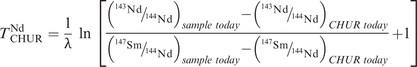
where λ is the decay constant for 147Sm to 143Nd (Table 6.1). Both the preferred and historical values used to calculate CHUR are given in Table 6.3b. Care must be taken in selecting which CHUR value to use because different values have been reported in the past and if data are to be compared, they need to be normalized to the same CHUR values. Model ages are also sensitive to the difference in Sm/Nd between the sample and CHUR, and only fractionated samples with Sm/Nd ratios which are sufficiently different from the chondritic value will yield precise model ages.
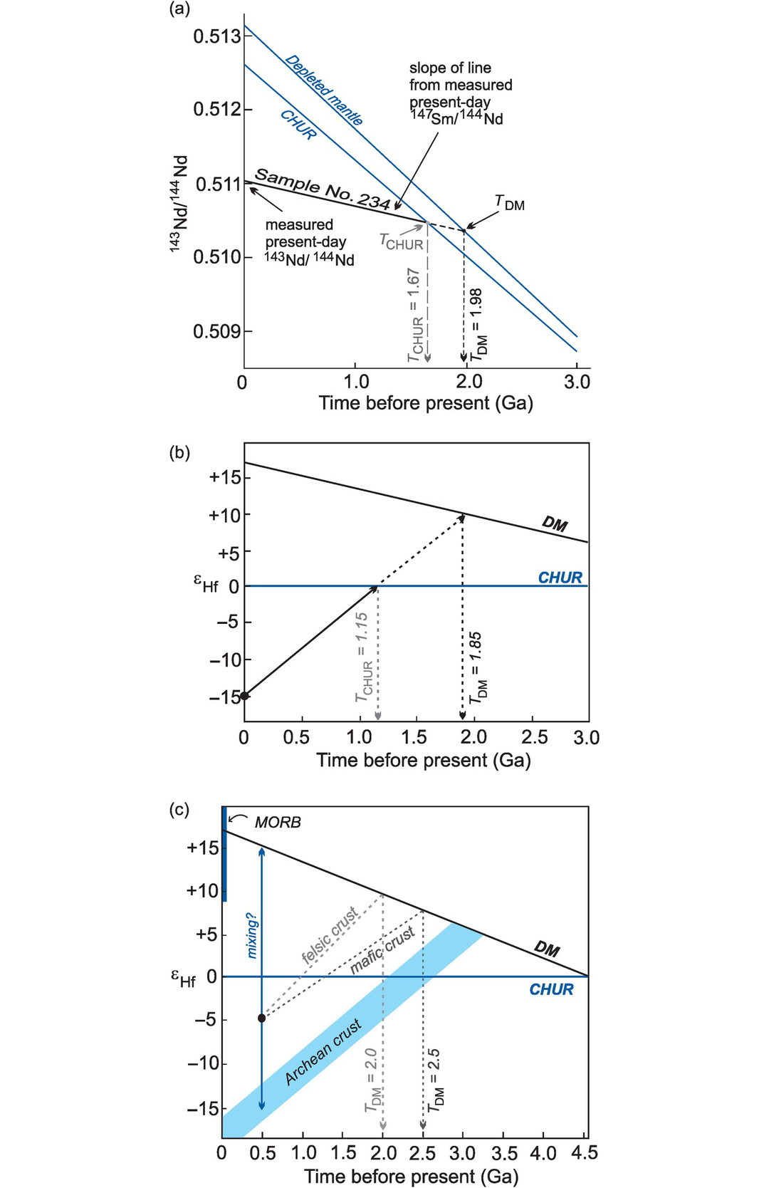
The calculation of Nd and Hf model ages. (a) The evolution of 143Nd/144Nd over time for sample 234 (Table 6.4) compared with two models of the mantle: CHUR (the chondritic uniform reservoir) and DM (the depleted mantle). A Nd model age is the time at which the sample had the same 143Nd/144Nd ratio as its mantle source. In this case there are two possible solutions depending upon the preferred mantle model. The TCHUR model age is approximately 1.67 Ga and the TDM model age is approximately 1.98 Ga. A similar diagram can be constructed using the epsilon notation (Section 6.3.4) in place of 143Nd/144Nd. (b) The evolution of 176Hf/177Hf expressed in εHf units (see Section 6.3.4) versus time. The Hf model age is the time at which the sample had the same 176Hf/177Hf ratio as its depleted mantle source. In this example the whole-rock 176Hf/177Hf measured today (εHf = −15) is extrapolated back through time until it intersects the model mantle composition of interest, providing the model age (THfCHUR = 1.15 Ga; THfDM = 1.85 Ga). (c) The evolution of εHf versus time and Hf-in-zircon model ages (modified from Kemp and Hawkesworth, 2014; with permission from Elsevier). Three different scenarios are shown for a zircon crystallised from a melt at 500 Ma with an εHf = −5. (i) The zircon crystallised from a melt that was derived from older mafic crust producing THfDM = 2.5 Ga; (ii) the melt was derived from an older felsic continental crust producing THfDM = 2.0 Ga; (iii) the melt was derived from a mixture of juvenile mantle melt and melt extracted from a heterogeneous Archean crust (dashed arrow) – in this case the model age has no significance. Also note the variation in depleted mantle composition as recorded by MORB (εHf = +8 to +22) compared with the assumed DM model composition. In the absence of other constraints, all scenarios can generate significantly different model ages.
| DMb | BSEb | CHURc | S-CHURd | |
|---|---|---|---|---|
| 87Rb/86Sr | 0.085 | 0.061 | ||
| 87Sr/86Sr | 0.7026 | 0.7045 | 0.7047 | 0.7030 |
| Rb (ppm) | 600 | 430 | ||
| 147Sm/144Nd | 0.1960 | 0.2082 | ||
| 143Nd/144Nd | 0.51311 | 0.512634 | 0.512630 | 0.512990 |
| 176Lu/177Hf | 0.0336 | 0.0375 | ||
| 176Hf/177Hf | 0.28330 | 0.282843 | 0.282785 | 0.28313 |
| 187Re/188Os | 0.40186 | |||
| 187Os/188Os | 0.1276e |
| Nd isotopes | DePaolo; Wasserburgb | O'Nions; Allegre; Hawkesworthb | ||||||
|---|---|---|---|---|---|---|---|---|
| Normalising factors | ||||||||
 | = 0.636151 [1], = 0.63613 [2] |  | = 0.63223 [3] | |||||
 | = 0.2096 [1], = 0.209627 [4] |  | = 0.7219 [3] | |||||
| Chondritic Uniform Reservoir | ||||||||
 | = 0.505829 [1] | Sm/Nd = 0.31 [5] = 0.50677 ? 10 [6] | ||||||
 | = 0.511847 [4], = 0.511836 [7] | = 0.51262 [8] | ||||||
 | = 0.1967 [1] | = 0.1966 [9], = 0.1967 [10], = 0.19637-0.1968 [11] | ||||||
| Depleted mantle | ||||||||
 | = 0.51235 [7], = 0.512245 [12] | = 0.51315 [10], = 0.51316 [9] | ||||||
| = 0.513114 [13], = 0.51317-0.51330 [11] | ||||||||
 | = 0.214 [7], = 0.217 [14] = 0.225 [15], = 0.23 [12] | = 0.2137 [10], = 0.222 [13], = 0.233-0.251 [11] | ||||||
| International rock standard BCR-1 | ||||||||
 | = 0.51184 [16] | = 0.512669 ± 8 [17] | ||||||
| Basaltic achondrite best initial (BABI) | ||||||||
| 87Sr/86Sr(4.6 Ga) | = 0.6998 [18] | |||||||
a Assuming λ = 6.54 × 10⁻¹² yr−1.
b References: [1] Jacobsen and Wasserburg (1980); [2] DePaolo (1981a); [3] O’Nions et al. (1977); [4]Wasserburg et al. (1981); [5] O’Nions et al. (1979); [6] Lugmair et al. (1975); [7] McCulloch and Black (1984); [8] Hawkesworth and van Calsteren (1984); [9] Goldstein et al. (1984); [10] Peucat et al. (1988); [11] Allegre et al. (1983); [12] McCulloch and Chappell (1982); [13] Michard et al. (1985); [14] Taylor and McLennan (1985); [15] McCulloch et al. (1983); [16] DePaolo and Wasserburg (1976); [17] Hooker et al. (1981); [18] Hans et al. (2013).
Currently, there is some debate over whether the Earth’s mantle had a chondritic or a supra-chondritic (S-CHUR) composition. Caro and Bourdon (2010) provide an overview of the arguments in favour of S-CHUR and from studies of the short-lived Nd isotope 142Nd argue that the non-chondritic 142Nd/144Nd of the Earth implies a non-chondritic Sm/Nd for the Earth. Their S-CHUR values are given in Table 6.3a, and S-CHUR model ages can be determined in the same way as TCHUR by simple substitution of S-CHUR values for CHUR values. It should also be noted, however, that the Earth’s mantle could have had a chondritic Sm/Nd but that this compositional component was sequestered at the base of mantle early in Earth’s history – in which case the CHUR model remains applicable.
The calculation of model ages for the Lu–Hf isotopic system uses the same principles as the Sm–Nd system. The Lu–Hf system also involves relatively insoluble, immobile and refractory elements (Lu, Hf), and therefore the Lu/Hf of Earth is also expected to be similar to chondrite. The evolution curve for a sample is constructed from the present-day (measured) values of 176Lu/177Hf and 176Hf/177Hf for the sample, calculated at some time (t) using the equation:
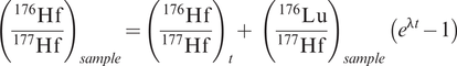
where λ is the decay constant for 176Lu to 176Hf, t is an arbitrarily selected time in the past to construct the evolution curve, and the subscript ‘sample’ denotes the measured, present-day ratio of the sample. The CHUR model age is calculated from the present-day 176Lu/177Hf and 176Hf/177Hf of a sample using the equation:
where λ is the decay constant for 176Lu to 176Hf (Table 6.1). This is illustrated in Figure 6.3b in which the present-day 176Hf/177Hf composition of the sample is extrapolated back in time until it intersects the CHUR evolution line, providing the CHUR model age. The values for CHUR are given in Table 6.1. In Figure 6.3b the Hf isotope values are expressed in εHf units – this is an alternative way of expressing an isotope ratio relative to CHUR. The ε notation is frequently applied to both Hf and Nd isotopes and is discussed more fully in Section 6.3.4. As in the case of Nd isotope model ages, when compiling data it is necessary to check that all the data are normalized to the same CHUR value.
6.2.2.2 Depleted Mantle Model Ages (TDM)
Studies of initial 143Nd/144Nd (often denoted with the subscript i) from Precambrian terrains suggest that the mantle which generated the continental crust has evolved since earliest times with a Sm/Nd ratio greater than that of CHUR. Consequently, model ages for the continental crust are usually calculated with reference to the depleted mantle (DM) reservoir rather than CHUR. Depleted mantle model ages are calculated by substituting the values for (143Nd/144Nd)CHUR today with (143Nd/144Nd)DM today and (147Sm/144Nd)CHURtoday with (147Sm/144Nd)DMtoday into Eq. 6.5. Similarly, Hf depleted mantle model ages are calculated by substituting the appropriate DM values into Eq. 6.7 such that (176Hf/177Hf)CHURtoday and (176Lu/177Hf)CHURtoday become (176Hf/177Hf)DMtoday and (176Lu/177Hf)DMtoday. The appropriate values are given in Table 6.3 and a graphical solution of a TDM model age calculation for both the Nd and Hf systems (using the epsilon notation – see Section 6.3.4) is illustrated Figure 6.3a, b.
6.2.2.3 Hf Depleted Mantle Model Ages Calculated for Zircon
Hf model ages (or crustal residence ages; see Section 6.2.3.2) can also be calculated for the mineral zircon and are used to trace crustal evolution – see, for example, Kemp and Hawkesworth (2014) for an excellent overview. Zircon has a very low Lu/Hf (<0.002) and therefore a low in-growth of radiogenic 176Hf and so preserves the near-initial 176Hf/177Hf inherited from its source at the time it crystallised. For the simplest scenario, that of an igneous zircon with a U–Pb crystallisation age the same as its Hf model age, the U–Pb age directly dates the time at which the host melt was extracted from its (depleted) mantle reservoir. These ages therefore reflect the timing of the formation of new crust, although it is important to note that there is some uncertainty over the 176Hf/177Hf of the depleted mantle (Chauvel and Blichert-Toft, 2001).
However, in contrast to the simple scenario outlined above, many zircon U–Pb ages are significantly younger than their THfDM ages and may differ by several hundred million years (Figure 6.3c). In this case, the interpretation of Hf model ages can be much more ambiguous. This uncertainty arises because zircon sequesters Hf more strongly than Lu, and so the Lu/Hf in zircon is not easily converted into Lu/Hf of the parent magma. Further, as shown in the εHf versus time plot in Figure 6.3c, the mixing between a magma and a melt derived from source rocks containing zircons of different ages will provide a calculated model age without geological significance. There is also a range of possible DM growth curves which will affect both Nd and Hf model ages. These are discussed more fully in Section 6.3.3.
6.2.2.4 Assumptions in the Calculation of Model Ages
When calculating a model age it is important to ensure that the assumptions on which the calculation is based are fulfilled. The first major assumption is that of the composition of the isotopic reservoir which is being sampled, for this could be S-CHUR, CHUR or DM. This is important because there can be as much as 300 Ma difference between TCHUR and TDM Nd model ages as illustrated in Figure 6.3a. A further concern is that there are several different models for the depleted mantle source. Three of these are illustrated in Figure 6.14b below using the εNd notation (the deviation of the isotopic composition from CHUR) and it is important therefore that the model being used for the depleted mantle is specified. There are also a number of different normalisation schemes in use for the Nd isotope system. These are listed in Table 6.3b. It is important therefore that when calculating model ages or plotting data from different sources the same set of normalising values is used consistently.
A second major assumption used in model age calculations is that the parent/daughter element ratio of the sample has not been modified by fractionation after its separation from the mantle source. A third assumption is that all material is extracted from the mantle was derived in a single event. Examples of Nd–model age calculations using Eq. 6.5 for TNdCHUR and TNdDM for a suite of metamorphic rocks from central Australia are given in Table 6.4.
| Sample no. |  |  | TNdCHUR (Ga) | TNdDM (Ga) |
|---|---|---|---|---|
| Mafic granulites | ||||
| 226 | 0.1853 | 0.511772 ± 36 | 0.856 | 2.203 |
| 234 | 0.1251 | 0.511049 ± 30 | 1.672 | 1.975 |
| 551 | 0.2134 | 0.512122 ± 36 | 2.596 | 2.950 |
| 868 | 0.2046 | 0.512013 ± 24 | 3.388 | 2.491 |
| Quartzofeldspathic and calc-silicate rocks | ||||
| 501A | 0.1248 | 0.511006 ± 28 | 1.755 | 2.034 |
| 507 | 0.1310 | 0.511039 ± 24 | 1.844 | 2.115 |
| 503 | 0.1248 | 0.510967 ± 32 | 1.837 | 2.093 |
| 512 | 0.1150 | 0.510794 ± 32 | 1.938 | 2.145 |
6.2.3 Important Concepts in Geochronology
6.2.3.1 Closure Temperature (Tc)
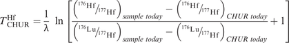
One of the principal controls on the retention of a radiogenic daughter product in a mineral is temperature, and so it is important to know the point at which a rock or mineral becomes a closed system with respect to retention of a particular daughter isotope. This temperature is known as the closure or blocking temperature (Tc) (Figure 6.4). The concept of closure temperature was defined by Dodson (1973, 1979) as ‘the temperature of a system at the time of its apparent age’. A more recent discussion of this topic in the context of a wider discussion of thermochronology is given by Reiners et al. (2018).
The Tc of a mineral depends on the thermally activated diffusion or annealing of radioisotopic daughter products, which in turn is a complex function of composition, grain size, grain shape, activation energy, cooling rate and whether or not a fluid is present to facilitate diffusion. For this reason, different minerals close at different temperatures and a single mineral will have a different Tc for each isotopic system (Table 6.5). It is unlikely, therefore, given the number variables that control the Tc, that there is a specific Tc for a given mineral associated with a particular isotopic system (Reiners, 2009; Cassata et al., 2011; Cassata and Renne, 2013). Even so, the cooling rate seems to exert the strongest influence on Tc, with a higher cooling rate generally producing a higher Tc (Figure 6.5). With this caveat in mind, Tc is most commonly used to describe minerals, and the Tc measured in several different minerals from a single rock may help to define the cooling history of that rock (Figure 6.6).
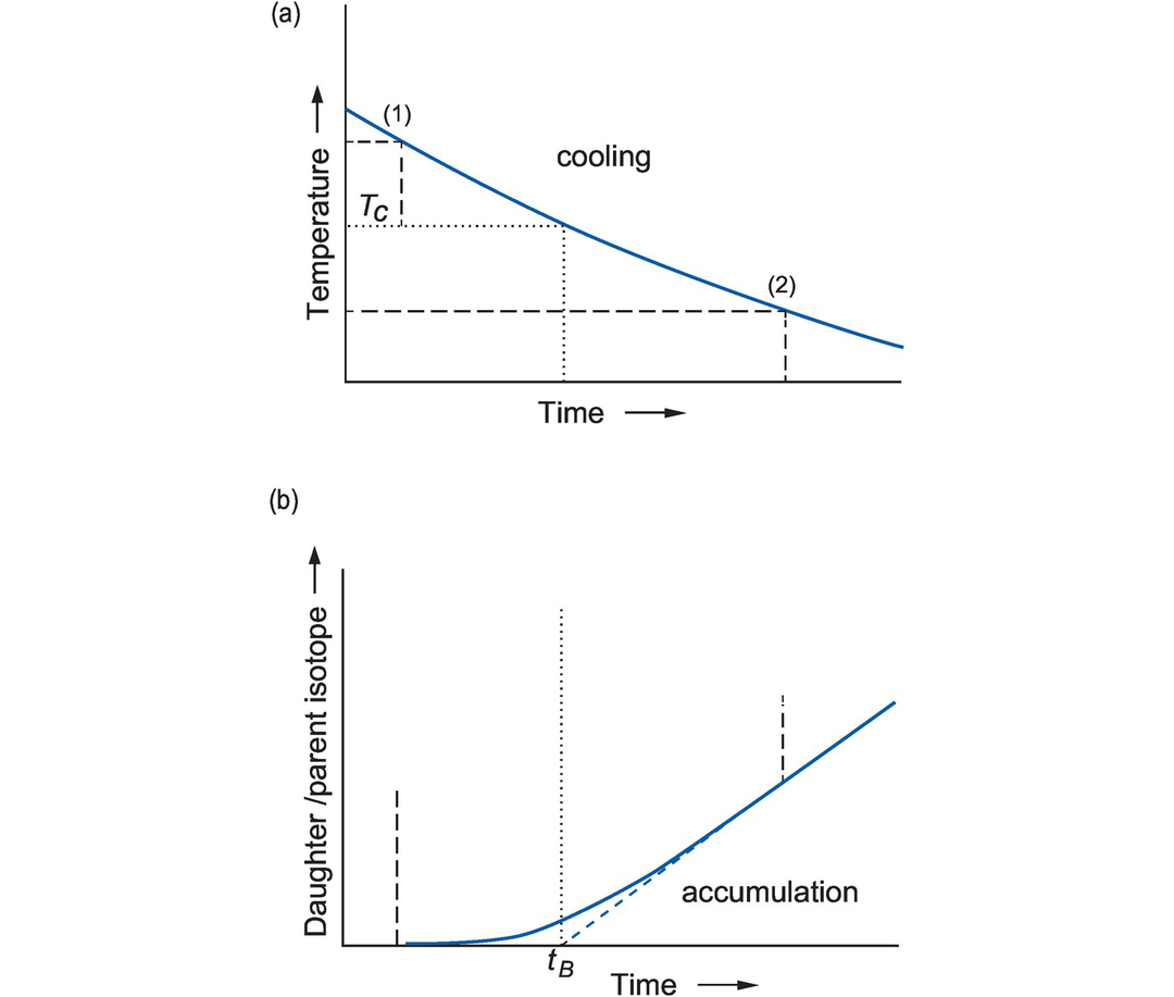
Closure (or blocking) temperature (after Dodson, 1979). (a) The cooling curve as a function of time. When a mineral is near its temperature of crystallisation (1) the daughter isotope will diffuse out of the mineral as fast as it is produced and cannot accumulate. As cooling continues, the mineral enters a transitional stage (between (1) and (2)) in which some of the daughter isotope is lost and some is retained, until finally at low temperatures the rate of escape is negligible and the daughter isotope is retained (2). (b) The accumulation curve of the concentration of the daughter to parent isotope as a function of time. The ‘age’ of the system (tB) is an extrapolation of the accumulation curve to the time axis (blue dashed line). The closure temperature (Tc) is the projection of this point onto the cooling curve in (a) (dotted line). Tc depends partly upon the cooling rate of the system but is independent of the starting temperature if the latter is sufficiently high. In a specific isotopic system, fast cooling rates have a higher Tc, while lower cooling rates have a lower Tc.
| Mineral | Reference | Tc (°C) |
|---|---|---|
| U–Th–Pb isotopic system | ||
| Monazite | Cherniak et al. (2004) | 1018 |
| Zircon | Cherniak and Watson (2001) | 974 |
| Rutile | Cherniak (2000) | 624 |
| Titanite | Cherniak (1993) | 645 |
| Apatite | Cherniak et al. (1991) | 473 |
| Lu–Hf isotopic system | ||
| Zircon | Cherniak et al. (1997)b | >900 |
| Garnet | Scherer et al. (2000) | ≥GtNd |
| Sm–Nd isotopic system | ||
| Diopside | Cherniak et al. (1997) | >750 |
| Titanite | Cherniak et al. (1997) | >700 |
| Garnet | Ganguly et al. (1998) | 690 |
| Apatite | Cherniak et al. (1997) | 400–1000 |
| Rb–Sr isotopic system | ||
| Biotite | Hammouda and Cherniak (2000) | 581 |
| Muscovite | Jenkin (1997) | 521 |
| Plagioclase | Jenkin et al. (1995) | 521 |
| K-feldspar | Cherniak and Watson (1992) | 396 |
| 40Ar/39Ar isotopic system | ||
| Hornblende (magnesian) | Harrison (1981) | 569 |
| Phlogopite | Giletti (1974) | 459 |
| Muscovite | Robbins (1972) | 393 |
| Biotite | Grove and Harrison (1996) | 358 |
| K-feldspar (low sanidine) | Wartho et al. (1999) | 357 |
| K-feldspar (orthoclase) | Foland (1994) | 222 |
| Maskelynite | Weiss et al. (2002) | 6 |
| (U–Th)/He isotopic system | ||
| Magnetite | Blackburn et al. (2007) | 247 |
| Titanite | Reiners and Farley (1999) | 212 |
| Monazite | Farley (2007) | 200 |
| Olivine | Shuster and Farley (2005) | 187 |
| Zircon | Reiners et al. (2004) | 184 |
| Xenotime | Farley (2007) | 176 |
| Epidote | Nicolescu and Reiners (2005) | 86 |
| Apatite | Farley (2000) | 69 |
| Goethite | Shuster et al. (2005) | 51 |
| Quartz | Shuster and Farley (2005) | 48 |
| Basaltic glass | Kurz and Jenkins (1981) | 24 |
| Fission track | ||
| Zircon | Rahn et al. (2004) | 342 |
| Apatite | Ketcham et al. (1999) | 115 |
| Fission track, He | ||
| Apatite, 4He 103 nmol/g | Shuster et al. (2006) | 109 |
| Apatite, 4He 102 nmol/g | Shuster et al. (2006) | 87 |
| Apatite, 4He 10 nmol/g | Shuster et al. (2006) | 69 |
| Apatite, 4He 1 nmol/g | Shuster et al. (2006) | 58 |
| Apatite, 4He 10−1 nmol/g | Shuster et al. (2006) | 53 |
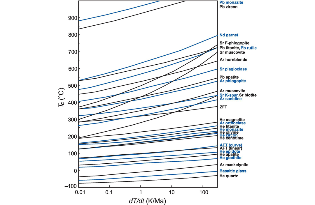
The closure temperature (Tc) of some common minerals as a function of cooling rate (after Reiners et al., 2018; with permission from John Wiley & Sons). Note that fast cooling rates have higher Tc. The isotopic system and mineral are specified on the right-hand axis. ZFT, zircon fission track; AFT, apatite fission track.
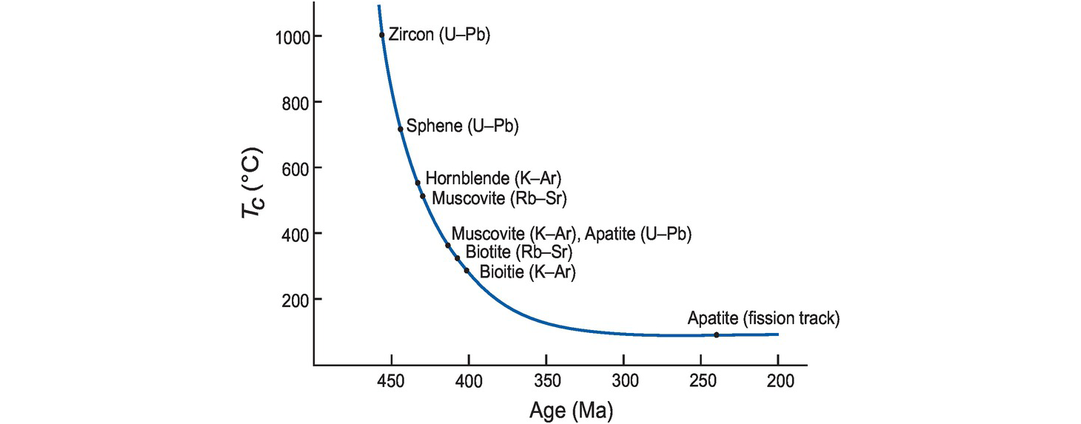
The cooling history of the Glen Dessary syenite, Scotland (after Van Breemen et al., 1979, and Cliff, 1985). Mineral age is plotted against approximate Tc (with mineral and method indicated). The combination of different minerals and isotopic systems define a range of Tc and produce ‘cooling’ ages; these define the cooling history for the pluton which can be expressed as °C/Ma.
A distinction must be made between closure temperature and the resetting of an isotopic system. The latter will take place in samples which have been thermally overprinted and/or subject to fluid flow, and normally it is the process of fluid interaction that is more influential in resetting an isotopic system than temperature alone. Choosing between closure temperature (mainly controlled by volume diffusion) and the resetting of an isochron (most commonly a function of fluid flow) to explain discordant isotopic ages requires a consideration of the scale of isotopic homogenisation. For example, rocks which have been isotopically reset may yield a range of ages that vary from the time of crust formation to the most recent metamorphic event, and this may depend upon the scale of sampling such that large samples may escape isotopic re-homogenisation and preserve old ages, whereas individual minerals may have recrystallised and yield younger ages. In the following section we shall look more closely at the meaning of the term ‘age’ in the light of the Tc concept and discuss the different ways it has been used in both mineral and whole-rock systems.
6.2.3.2 What Is an ‘Age’?
In geochronology we distinguish between a ‘date’ and an ‘age’. The former is used to describe an analytical result that has not yet been interpreted or given any geochronological significance. The term ‘age’ is used when applied to the results of an isochron calculation or a model ‘age’ calculation on a whole rock or a mineral sample once the geological significance of the result has been evaluated. The meaning of the term ‘age’ is always a matter of interpretation, for there are a number of different processes that can impart geological significance to a calculated ‘age’. For this reason, the term ‘age’ is best used with an additional qualifying term. These are discussed below.
(a) Crystallisation age. The crystallisation age of a mineral or a rock records the time at which it crystallised. In an igneous rock the crystallisation age of a mineral records the magmatic age of the rock. In the case of a metamorphic mineral, if the temperature of crystallisation is lower than the closure temperature, the instant the mineral forms it records its age of crystallisation.
(b) Metamorphic age. A metamorphic age is the time of peak metamorphism. This is different from the cooling age, which is discussed below. A metamorphic age depends upon the metamorphic grade. In low-grade metamorphic systems the metamorphic maximum may be determined from the blocking temperature of a specific mineral. In the case of high-grade metamorphism, the time of the peak of metamorphism can be inferred from the resetting of a whole-rock system such as Rb–Sr or Pb–Pb or the timing of new zircon growth (Figure 6.8).
(c) Cooling age. In a metamorphic rock the term ‘cooling age’ describes the time, after the main peak of metamorphism, when for a given isotopic system a mineral passes through its closure temperature. In an igneous rock the cooling age is the time after solidification of the melt that a mineral passes through its closure temperature. A cooling age therefore must be specified in terms of both the isotopic system and the mineral (Figure 6.5).
(d) Crust formation age. A crust formation age represents the time at which new continental crust is extracted from the mantle (O’Nions et al., 1983). Normally, the genesis of new continental crust is followed by deformation, metamorphism and melting, and so it is not always possible to easily determine the age of crust formation, only the timing of the later metamorphism and/or partial melting.
(e) Crustal residence age. The term ‘crustal residence age’ applies to sediment derived from an area of continental crust and reflects the age of that crust (Figure 6.7). A Nd crustal residence age (Tcr) is calculated from Eq. 6.5 by substituting appropriate values for the depleted mantle DM (the original source of the continental crust) in place of the values for CHUR. Some authors use the term ‘provenance age’ instead of crustal residence age, although this should not be taken to signify a specific event such as stratigraphic age, but rather is the average crustal residence time of all the components of the rock. Typically, the crustal residence age of a sedimentary rock is older than its stratigraphic age (Figure 6.7).
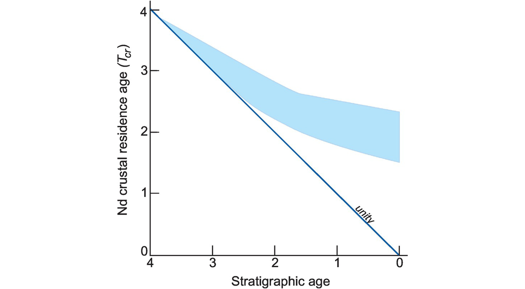
Crustal residence age (Tcr) diagram. Stratigraphic age is plotted against neodymium Tcr for fine-grained clastic sediments from 4.0 Ga to the present day (shaded region). The departure from the 1:1 line at about 2.5 Ga shows that Archaean sediments contain a mainly juvenile component, whereas Phanerozoic sediments contain an old crustal component.
6.2.4 Whole-Rock versus Mineral Age?
Choosing between a whole-rock or mineral age determination depends on the nature of the investigation. Useful age information may be extracted from whole rock systems as follows:
In rapidly cooled volcanic rocks, it is possible to measure the time of crystallisation.
In metamorphic rocks, whole-rock data can be used to measure the time of peak metamorphism.
In some instances, whole-rock model ages can be used to determine the time of crust formation.
Isotopic measurements of minerals can be used in mineral isochron calculations to determine individual mineral ages or the cooling history of a rock (see Section 6.2.3.1). Highly refractory minerals such as zircon with a high Tc can provide magmatic crystallization ages and sometimes even after multiple metamorphic events may preserve the time of crust formation. Minerals preserved as inclusions within refractory phases such as zircon, garnet or diamond can be protected from later overprinting events and may record the very early history or even the prehistory of the parent rock (e.g., Delavault et al., 2016).
The advent of analytical tools which permit the in situ, high spatial resolution measurement of isotope ratios in individual mineral grains has revolutionised geochronology (Compston, 1984; Košler et al., 2002). Not only can multiple analyses be made on a single crystal, helping to unravel the geological history of complex mineral grains, but the low-sampling volume associated with SIMS analysis permits multiple methods to be applied to the same analytical domain. For example, it is common to determine both the U–Pb age and the Hf isotope model age from within a single growth zone of a zircon crystal (Robinson et al., 2019) or both the U–Pb age and the REE chemical composition at the same analytical position in a single grain of zircon or garnet (Whitehouse and Platt, 2003).
6.2.5 Isotopic Systems Used in Geochronology
The reader should refer to Table 6.1 for the details of the radioactive decay schemes discussed in the sections below.
6.2.5.1 The K–Ar and Ar–Ar Systems
Within the family of the longer-lived radiogenic isotope systems used for dating geological events, 40K has one of the shortest half-lives. In addition, potassium is abundant in crustal rocks, whereas the concentration of the volatile noble gas Ar in the Earth is low, and so the Earth has a high 40K/40Ar ratio. For these reasons, the K–Ar system is the preferred method for accurately dating young events in fresh igneous rocks and, because of the volatility of Ar, measuring the time of reheating in igneous and metamorphic rocks. K–Ar ages are precise to about 30,000 years.
The 40Ar/39Ar method was developed from the K–Ar method. 39Ar does not occur naturally but is produced by irradiating a K-bearing sample with fast neutrons to produce 39K (half-life of 269 years). The amount of 39Ar produced is therefore a function of the amount of 39K present in the sample. Since at any point in the Earth’s history the 40K/39K ratio is constant, the amount of 40K present in the sample can also be calculated from the 39Ar measured. This forms the basis of 40Ar/39Ar dating.
Argon isotopes are most commonly measured in K-bearing minerals such as biotite, muscovite, K-feldspar and hornblende. The Tc associated with these minerals is in the ‘mid-temperature’ range (Tc = 200–550°C, Figure 6.5). At these temperatures, the closure temperature is highly dependent on the length scale of diffusion and the grain size and shape (Cassata et al., 2011; Cassata and Renne, 2013). This means that, depending on cooling rate, closure temperatures can vary by as much as ~200°C (Figure 6.5). Nonetheless, useful age data can be obtained from both K–Ar and 40Ar/39Ar methods and provide crystallization ages for rapidly cooled rocks, cooling ages in slowly cooled rocks (Rose and Koppers, 2019) and the time of diagenesis in sediments (Schomberg et al., 2019). Frequently, geochronological data are collected using a step heating method in which the cumulative 39Ar released is used to produce an age spectrum. Modern laser ablation systems allow micron-level spatial resolution of argon isotope measurements, and the in situ measurement of volcanic glass and minerals has been successfully applied using ~100-μm analytical spots (Warren et al., 2012).
6.2.5.2 The Rb–Sr System
The elements Rb and Sr are sufficiently abundant in most crustal rocks (10–1000 ppm) for the Rb–Sr method of geochronology to be useful in a wide range of rock types and minerals. However, Rb and Sr are also relatively mobile and the Rb–Sr isotopic system is frequently disturbed by the influx of fluids or by later thermal events. Consequently, Rb–Sr dating requires pristine samples and is rarely useful for constraining crust formation ages. Nevertheless, a Rb–Sr isochron has meaning and can usually be attributed to an event such as the time of metamorphism or recystallisation in an igneous rock or the time of diagenesis in a sedimentary rock.
The Rb–Sr method is often applied to the minerals biotite, muscovite, plagioclase K-feldspar and apatite. Ages can be calculated from a two-point isochron method in which a mineral with a low concentration of Rb such as plagioclase feldspar is used as a control on the initial ratio of the rock. Alternatively, mineral ages can be determined from single crystals or even parts of single crystals associated with specific metamorphic fabrics (Cliff et al., 2017).
6.2.5.3 The U–Th–Pb/He System
The utility of the U–Th–Pb system lies in its independent and branching decay schemes and in the contrasting geochemical properties of the elements involved. U and Th are actinides, incompatible and refractory. Under oxidizing conditions U exists as U6+ and can be highly mobile. Pb is slightly less incompatible, is chalcophile and exists in several oxidation states.
The focus here is on the Pb–Pb, 235U–207Pb and 238U–206Pb systems. U-series dating, which involves the numerous intermediate to short-lived daughter products within the U–Th–Pb system, is useful for dating very young geological processes but is not addressed here. Nor are the methods of the He fission track system that is used to determine the timing of low-temperature process associated with erosion. For a thorough discussion of these systems, we refer the interested reader to White (2015) and Reiners et al. (2018).
Pb–Pb whole-rock and mineral isochrons can be plotted for a wide range of rock types from granites to basalts, and can also be used to determine the depositional age of some sediments. The method yields reliable ages in rocks with simple crystallisation histories. However, the differences in U and Pb mobility and geochemical behaviour may complicate the interpretation if the isotopes have been reset. Thus, the Pb–Pb isochron method rarely provides crust formation ages and is better used to determine the age of metamorphism.
The combined use of the 206Pb/238U and 207Pb/235U systems allows an assessment of whether the assumptions associated with Tc have been met. This approach is commonly applied to mineral samples such as zircon. When samples which have had an undisturbed thermal history are plotted on a 206Pb/238U versus 207Pb/235U plot, they should lie on the ‘concordia’ curve (Figure 6.8). The concordia curve is the theoretical curve along which a series of 238U and 235U ages over time are the same (Figure 6.8, Box 6.1) and is calculated from the decay constants of the two systems. Hence a U-, Th-, Pb-bearing mineral population may define a linear array on a concordia diagram with an upper and lower time intercept on the concordia curve (Figure 6.8). The normal interpretation of the linear array, known as the discordia, is one of lead loss (or uranium gain) in which its upper and lower intercepts with the concordia curve may have petrological significance.
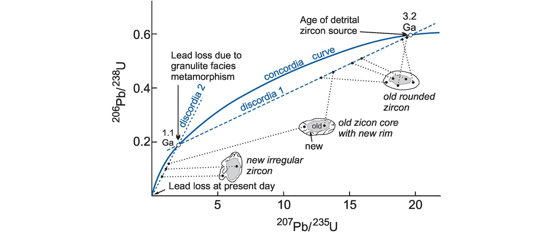
U–Pb concordia diagram. 207Pb/235U and 206Pb/238U data from zircon grains from a granulite facies metasediment from Sri Lanka (after Kroner et al., 1987). The concordia curve defines the theoretical evolution through time of 206Pb/238U and 207Pb/235U ages that are equivalent (Box 6.1). It is curved because 235U and 238U have different half-lives. A discordia is a line fitted to data points that are not concordant (do not coincide with the concordia curve). A discordia may intersect the concordia curve at two points. The sketches show morphologies of individual zircon grains and the locations analysed using a secondary ion mass spectrometer (SIMS). Old zircon grains and the cores of composite grains define a linear array (discordia 1) with an upper intercept at 3.2 Ga and a lower intercept at 1.1 Ga. The upper intercept is interpreted as the age of the source of detrital zircon and the lower intercept as the time of granulite facies metamorphism. New zircon grains (recognised on the basis of their irregular morphology) and new zircon overgrowth on composite grains define a second linear array (discordia 2) with an upper intercept at 1.1 Ga (the time of granulite facies metamorphism) and a lower intercept at the present day. The new zircon growth was interpreted to have occurred during the granulite facies event.
U and Th typically occur in zircon, monazite, rutile, titanite, epidote and apatite and so are often used in U–Th–Pb isotopic studies. Zircon in particular is a highly refractory mineral and so is especially useful since it can retain primary (crystallization) age information despite being affected by secondary processes (e.g., Reimink et al., 2016, and references therein). Thus, magmatic zircons in felsic rocks may be used to date the time of crystallisation from the upper intercept of the discordia curve. In contrast, granitic rocks which are melts of older crust may contain inherited (xenocrystic) zircons and in this case the lower intercept may represent the age of crystallisation, while the upper intercept may reflect the age of the crustal source (Amelin et al., 2000). In sediments, detrital zircons can reflect the age and composition of the sediment source (Zhang et al., 2015), and in metamorphic rocks zircons are used to date the age of the protolith and also the time of metamorphism (Hoiland et al., 2018). The application of high spatial resolution methods allows the dating of mineral growth zones within a single zircon grain and identification of the magmatic and, if applicable, the metamorphic chronology of the rock (Figure 6.8).
6.2.5.4 The Sm–Nd System
The REE elements Sm and Nd are incompatible and therefore are more abundant in the crust than in the mantle. They are less mobile than Rb, Sr, Th, U and Pb and so may preserve ‘original’ isotopic signatures in rocks whose Rb–Sr and Pb isotopic chemistry has been disturbed. The Sm–Nd isotope system is important in dating mafic rocks and meteorites where there is sufficient Sm/Nd fractionation to allow the accurate determination of an age and is one of the best methods for obtaining crust formation ages from a whole-rock analysis.
The chief limitations of the Sm–Nd method are associated with its long half-life, which restricts its application to older rocks, and the relatively small variations in Sm/Nd found in most cogenetic rock suites. For this reason, some workers have combined different lithologies on an isochron diagram to obtain a wider spread of Sm/Nd ratios, although this strategy requires a clear demonstration of their cogeneticity; otherwise, samples extracted from different sources and with very different histories will generate a questionable isochron.
Some accessory minerals such as apatite, monazite, sphene or garnet fractionate the REE and are useful in Sm–Nd mineral geochronology. Garnet is particularly important in this regard, for it has a high Tc (~500–700°C, Figure 6.5) and can be used to date the peak of metamorphism. Garnet-bearing mineral assemblages also offer the potential for precise Sm–Nd mineral isochron ages because garnet has a high Sm/Nd ratio which allows the slope of a mineral isochron to be accurately determined with errors of only 5–10 Ma for Mesozoic ages (Zheng et al., 2002; Lotout et al., 2020). Garnet ages are determined on two-point isochrons between garnet and whole-rock or one or more of the minerals plagioclase, pyroxene and hornblende with less fractionated Sm/Nd. Mineral isochrons which do not involve garnet are also possible but generally define a smaller range in Sm/Nd, although they may still yield ages with errors of ~20 Ma.
6.2.5.5 The Lu–Hf System
The Lu–Hf system is similar to the Sm–Nd isotopic system inasmuch as Lu is also a REE, but the half-life of 176Lu is shorter than 147Sm (37 Ga versus 106 Ga). This means that Lu/Hf and therefore 176Hf/177Hf in rocks and minerals should have a greater range than is seen by 143Nd/144Nd in the Sm–Nd system. Theoretically, the Lu–Hf method should permit precise isochron age determinations for older rocks. In practice, however, the lack of significant Lu/Hf fractionation in most crustal rocks and in common rock-forming minerals prevents this method from being used to determine isochron ages. Instead, the main applications are limited to those few specific minerals which fractionate Lu/Hf, as will be discussed in Section 6.3.1.2.
Lu is the heaviest of the REEs and it is especially accommodated in those phases that prefer the HREE. Garnet is an excellent example and most garnet species strongly partition Lu relative to the lighter REEs and Hf. In addition, Hf is chemically similar to Zr and is therefore concentrated in the mineral zircon. Although this is an advantage in simple igneous systems and allows the application of Lu–Hf and U–Pb dating methods to the same zircon grains, the different diffusion rates of trivalent Lu and tetravalent Hf cations means that interpreting the results for metamorphic rocks is not always straightforward (Bloch et al., 2020, and references therein).
An important application of the Lu–Hf method is in the study of clastic sediments. These tend to concentrate the heavy minerals such as garnet and zircon in which it is possible to apply multiple isotopic techniques including U–Pb, O, and Lu–Hf isotopes, as well as to analyse for trace elements and the REE. This means that in both modern and ancient sedimentary systems individual detrital mineral grains can be used to obtain information about both their source and the processes operating in the source region (Hoiland et al., 2017). When sufficient grains are analysed it is also possible to constrain their likely tectonic setting (Cawood et al., 2012).
6.2.5.6 The Re–Os System
In contrast to the highly lithophile elements of the Rb–Sr, Sm–Nd or Lu–Hf systems, the elements Re and Os are highly siderophile elements (HSE) and so are depleted in the silicate Earth and are present only at the ppb to sub-ppb levels. Both Re and Os are HSE elements, but Os is also a PGE and therefore is associated with ultramafic rocks, sulphides and arsenides. In mantle phases Re is moderately incompatible, whereas Os is highly compatible. This results in crustal rocks having elevated Re/Os ratios relative to the mantle. As noted above, the overall concentrations of Re and Os in the crust are low, but it is the strong fractionation of Re/Os and their enrichment in specific minerals that forms the basis of Re–Os geochronology.
Because crustal materials have very low concentrations of Re and Os, the application of the Re–Os system is restricted to samples enriched in Re and with high Re/Os. Re is particularly concentrated in molybdenite, to a lesser extent in Cu sulphides, and in black shales. This makes the Re–Os system useful in the study of iron meteorites, ore deposits, ultramafic rocks and hydrocarbons. Re–Os dating is based on the isochron method and combines related samples or minerals on an isochron (Kendall et al., 2006; Day, 2016). The method has also been used to date shales as young as 150 Ma (Cohen et al., 1999), and model ages in excess of 2 Ga have been calculated for Phanerozoic ophiolitic rocks (Meibom et al., 2002).
The Re–Os system has also been used to date mantle melt extraction events (Carlson, 2005). Os is compatible during mantle melting, whereas Re is moderately incompatible. Consequently, a melt residue will have lower Re and higher Os than either the fertile mantle or a mantle melt. This means that in residual peridotites the Re–Os system is less sensitive to contamination by migrating melts, thereby allowing whole rock mantle xenoliths to return useful chronological information on the timing of melt extraction.
6.2.5.7 Data Reduction Software Used in Geochronology
There are two free software packages commonly used for the reduction of geochronological data, Isoplot (Ludwig, 2009) and IsoplotR (Vermeesch, 2018b). Isoplot 4.15 (www.bgc.org/isoplot_etc/isoplot.html) is a PC-based add-on for Excel, and will work with some Mac Windows-enabling programs. Versions for older operating systems are also available. IsoplotR (www.ucl.ac.uk/~ucfbpve/isoplotr/) is a similar program written in R and can be used on-line or off-line with a computer that has R installed on it.
6.2.6 The Interpretation of Model Ages
A model age is an estimate of the time at which a sample separated from its mantle source region, and for igneous rocks and meta-igneous rocks this is a good estimate of the time of crust formation. However, as noted above in Section 6.2.2.4 a number of assumptions have to be made when calculating a model age.
In the case of Sr isotopes, none of these criteria is usually fulfilled with any certainty for either igneous rocks or sediments (Goldstein, 1988) and consequently model ages are not usually calculated for the Rb–Sr system. On the other hand, useful and meaningful model ages can be calculated for Nd, Hf and Os isotopes, although in each case the reference reservoir (CHUR or DM) must be specified and in the case of DM model ages the precise DM model evolution curve must also be defined.
Model ages for granitoids may be used to estimate the age of their source. In the case of mantle-derived granites, the model age gives the time that the basaltic precursor to the granite was extracted from the mantle. This is often close in time to the crystallisation age of the granite. Granitoids which are derived by the melting of older continental crust give model ages which are indicative of the age of their crustal source, although this is realistic only when the parent/daughter element ratio has not been disturbed by fractionation. Often granites are a mixture of crustal and mantle sources. When this is the case calculated model ages provide only a minimum age (Arndt and Goldstein, 1987; Figure 6.9).
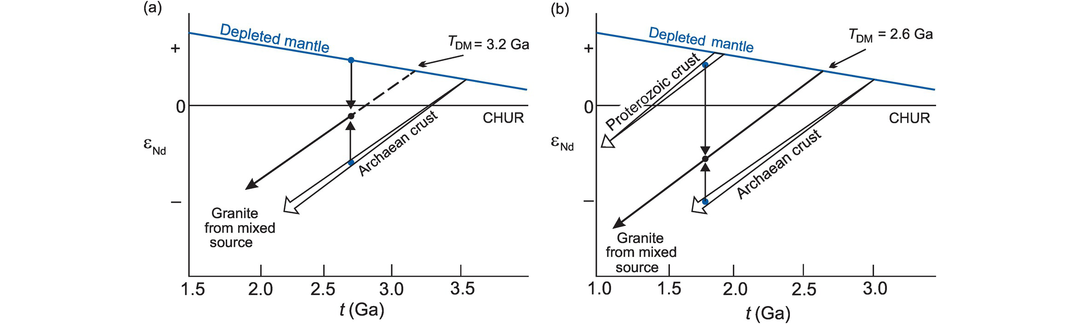
143Nd/144Nd evolution of the depleted mantle reservoir with time (in epsilon units; see Section 6.3.4). Relative to CHUR the depleted mantle shows increasing 143Nd/144Nd (increasingly positive εNd values) with time, whereas the continental crust shows retarded 143Nd/144Nd evolution (increasingly negative εNd values). (a) The depleted mantle model age for a granite formed at 2.7 Ga (black dot) from a mixture of a juvenile component derived from the depleted mantle and Archaean crust formed at 3.5 Ga will be 3.2 Ga. (b) The depleted mantle model age of a granite formed by the mixture of 1.9 Ga Proterozoic and 3.0 Ga Archaean crustal sources at 1.8 Ga will be 2.6 Ga. These diagrams show that model ages calculated for rocks with mixed sources provide only minimum ages of the crustal source.
Model ages for clastic sedimentary rocks provide an estimate of their crustal residence age (Section 6.2.3.2; O’Nions et al., 1983), again assuming minimal fractionation of the parent/daughter elements relative to the source. However, most continental sediment is a mixture of material from different sources. Consequently, model ages are likely to represent an average of the detrital input and provide only a minimum estimate of the crustal residence age or an average crustal residence age.
6.3 Using Radiogenic Isotopes in Petrogenesis
The mass difference between any pair of radiogenic isotopes is so small that the isotope pair cannot be fractionated by crystal–liquid processes. This means that during partial melting a magma retains the isotopic character of its source region and that isotope ratios remain unchanged during subsequent fractionation events.
These simple observations have led to two important developments in isotope geochemistry. First, source regions may have unique isotopic characteristics that can be defined, and, second, there may be mixing between isotopically distinct sources. Thus isotope geochemistry seeks to do the following:
A range of crust and mantle reservoirs is listed in Table 6.6 to demonstrate their isotopic variability. The larger and more difficult question of how the different crust and mantle reservoirs have acquired their isotopic signatures leads into the subject of crust and mantle geodynamics, a topic which treated briefly at the end of this chapter in Section 6.3.6.
| 87Rb–86Sr | 147Sm– 143Nd | 238U– 206Pb | 235U– 207Pb | 232Th– 208Pb | 176Hf/177Hf | 187Os/188Os | |
|---|---|---|---|---|---|---|---|
| Oceanic basaltic sources | |||||||
| DMMb | Low Rb/Sr | High Sm/Nd | Low U/Pb | Low U/Pb | Th/U = 2.4 ± 0.4 | 0.28330 | 0.1314–0.2316 |
| Low 87Sr/86Sr | High 143Nd/144Nd (positive εNd) | Low 206Pb/204Pb (~17.2–17.7) | Low 207Pb/204Pb (~15.4) | Low 208Pb/204Pb (~37.2–37.4) | |||
| HIMU | Low Rb/Sr | Moderate Sm/Nd | High U/Pb | High U/Pb | High Th/Pb | 0.28289 | 0.1305–0.1663 |
| low 87Sr/86Sr = 0.7029 | 143Nd/144Nd = <0.51282c | 206Pb/204Pb > 20.8 | high 207Pb/204Pb | (Mangaia) | |||
| EM-1 | Low Rb/Sr | Low Sm/Nd | Low U/Pb | Low U/Pb | Low Th/Pb | 0.28274 | 0.1342–0.1432 |
| 87Sr/86Sr (~0.705) | 143Nd/144Nd = <0.5112c | 206Pb/204Pb = 17.6–17.7 | 207Pb/204Pb = 15.46–15.49 | 208Pb/204Pb = 38.0–38.2 | (Gough) | ||
| EM-2 | High Rb/Sr | Low Sm/Nd | |||||
| 87Sr/86Sr > 0.722 | 143Nd/144Nd = 0.511-0.5121c | High 207Pb/204Pb and 208Pb/204Pb at a given 206Pb/204Pb | 0.282816 (Samoa) | 0.1173–0.1284 | |||
| Bulk Earth | 87Sr/86Sr = 0.7045 | 143Nd/144Nd = 0.512634 | 206Pb/204Pb = 15.58 ± 0.08 | 207Pb/204Pb = 18.4 ± 0.3 | 208Pb/204Pb = 38.9 ± 0.3 | 0.282843 | 0.1272–0.1303 |
| Continental crustal sources | |||||||
| Upper crust (sialic) | High Rb/Sr high 87Sr/86Sr | Low Sm/Nd low 143Nd/144Nd (negative εNd) | High U/Pb high 206Pb/204Pb | High U/Pb high 207Pb/204Pb | High Th/Pb high 208Pb/204Pb | 1.926 | |
| Mid crust | Semi-high Rb/Sr = 0.2–0.4 87Sr/86Sr = 0.72–0.74 | Crust shows retarded Nd evolution relative to chondritic source | U-depleted Low 206Pb/204Pb | U-depleted Low 207Pb/204Pb | Semi-high Th Semi-high 208Pb/204Pb | ||
| Lower crust (mafic) | Rb-depleted Rb/Sr < ~0.4 Low 87Sr/86Sr = 0.702–0.705 | Very U-depleted Very low 206Pb/204Pb (~14.0) | Very U-depleted Very low 207Pb/204Pb (~ 14.7) | Very Th-depleted Very low 208Pb/204Pb | 0.8040 | ||
a Disputed reservoirs are omitted (e.g., PREMA, FOZO, PHEM, C).
b Depleted MORB mantle.
c Normalized to 146Nd/144Nd = 0.7219.
Additional notes: 176Hf/177Hf from Salters and Stracke (2004) and Salters et al. (2011); 187Os/188Os MORB (Escrig et al., 2005), HIMU (Lassiter et al., 2003), EM-1 (Garapić et al., 2015), EM-2 (Jackson et al., 2016), BE (Van Acken et al., 2011, and references therein).
The isotopic variability between mantle sources may be thought of in terms of two separate processes. These are the process of mixing in which a number of different components contribute to the source, and the process of isotopic ingrowth in which the composition of the source evolves over geological time. Thus, radiogenic isotope ratios may be used to identify the separate components which have mixed to contribute to a particular magmatic suite such as in the case of the contamination of continental flood basalt with old continental crust. This mixing takes place over a relatively short time scale. In contrast, the isotopic evolution of a mantle source region as a function of the parent–daughter isotope ratio may take place over very long time scales – billions (Ga) rather than millions (Ma) of years.
Knowing how and when the different mantle sources acquired their separate identities is important for understanding the evolution of the Earth’s mantle, and it is this subject to which we now turn.
6.3.1 The Role of the Different Isotope Systems in Identifying Reservoirs and Processes
The elements used in geological radiogenic isotope studies vary greatly in their chemical and physical properties, so much so that different isotope systems vary in their sensitivity to particular petrological processes. This variability may show itself in three ways. First, the parent and daughter elements may under certain circumstances behave geochemically in different ways, such that the two become fractionated. For example, during mantle melting an element such as Rb is more readily concentrated in the crust than is the element Sr. The order of incompatibility for the elements of interest can be obtained from Figure 4.22 where the relative enrichments in MORB relative to the residual mantle and in the continental crust relative to MORB are shown.
A second possibility is that a parent–daughter element pair may behave coherently and so will not be fractionated, and yet behave in a very different manner from the parent–daughter pair of another isotopic system. For example, in the Sm–Nd and Lu–Hf systems the parent–daughter pairs share similar chemical and physical characteristics, whereas in the Re–Os, U–Th–Pb and Rb–Sr systems the parent–daughter pairs may be strongly fractionated relative to one another.
Finally, because of the geochemical similarity between the Sm–Nd and Lu–Hf isotope systems, it is reasonable to expect both systems to behave in a similar way and to display coupled geochemical behaviour. This is often evident on εNd versus εHf diagrams (Section 6.3.4). On occasion, the isotope systems display decoupled behaviour and this may also be of petrological significance.
We now briefly review some key geochemical properties of the Sr, Nd, Hf, Pb and Os systems. These are summarised in Table 6.6.
6.3.1.1 Sm–Nd Isotopes
In discussing the isotopes of Nd we differentiate between the long-lived Nd isotope system 147Sm→143Nd which is important in geochronology and the short-lived isotope system 146Sm→142Nd (half-life 103 Ma) which is relevant to our understanding of processes in the very early history of the Earth. The significance of the 146Sm→142Nd system is discussed more fully in Section 6.3.4.
The Sm/Nd ratio in the continental crust is lower than that of the depleted mantle and so over time generates lower 143Nd/144Nd ratios than are found in the depleted mantle. In this respect the Sm–Nd isotopic system is similar to Lu–Hf, but differs markedly from the U–Th–Pb, Rb–Sr and Re–Os systems. Since the elements Sm and Nd are not significantly fractionated after crust formation by subsequent metamorphic or sedimentary processes, Nd isotope ratios tend to preserve a memory of the parent–daughter isotope ratios of their source. In addition, Sm and Nd are immobile under hydrothermal conditions, and so Nd isotopes reflect the actual proportions of rock or magma involved in specific petrological processes, although this isotope system is insensitive to small amounts of recycled crust in the mantle.
6.3.1.2 Lu–Hf Isotopes
The Lu–Hf isotope system behaves in a similar way to the Sm–Nd isotope system. The Lu/Hf ratio in continental crust is lower than that in the mantle, and so with time the 176Hf/177Hf of the crust evolves to lower values relative to the Earth’s primitive mantle and the complementary depleted mantle evolves to higher values. A widespread and powerful application of Lu–Hf isotopes in petrology is the integration of Hf model ages with U–Pb crystallization ages for the mineral zircon. Recent studies have shown that in old continental crust, Hf model ages frequently exceed U–Pb zircon ages. This suggests that, if the U–Pb age represents the time of crystallisation of the crust, the Hf model age indicates an earlier event which is taken to be the time at which the precursor to the continental crust separated from the mantle (Kemp and Hawkesworth, 2014).
6.3.1.3 U–Th–Pb Isotopes
The U–Th–Pb system is more complex than other isotope systems used in geochemistry because it incorporates three independent decay schemes (Box 6.1) and because Pb isotopes do not define linear trends on lead isotope evolution diagrams. In terms of their geochemical behaviour U and Pb are incompatible in silicate minerals, although U enters a melt more readily than Pb, and U and Pb are relatively mobile in hydrothermal fluids, whereas Th is highly insoluble.
In detail the two isotopes of Pb produced from U decay (206Pb and 207Pb) show contrasting behaviour as a consequence of their differing radioactive decay rates (Box 6.1). Early in the history of the Earth 235U decayed rapidly relative to 238U, so that 207Pb evolved rapidly with time. Thus, 207Pb abundances are a sensitive indicator of an old source. Today, however, 235U is largely extinct so that in recent Earth history 238U decay is more prominent than that of 235U, and consequently the abundance of 206Pb shows a greater spread than 207Pb. This difference in behaviour between the Pb isotopes allows the identification of several isotopic reservoirs (Table 6.6). Crustal reservoirs are best sampled by studying the isotopic composition of a mineral with a low U/Pb or Th/Pb ratio such as feldspar for they preserve the ‘initial’ Pb isotopic composition of the source. This approach was developed by Doe and Zartman (1979), is now applied to single crystals using in situ analytical methods (Geng et al., 2020) and is discussed further in Section 6.3.6.1.
6.3.1.4 Rb–Sr Isotopes
During crustal melting the Rb–Sr isotope system has the greatest difference in compatibility between the parent and daughter elements. Rb and Sr are therefore easily separated and are strongly fractionated between crust and mantle. This results in the accelerated evolution of strontium isotopes in the continental crust relative to the mantle and with time has produced higher 87Sr/86Sr ratios than in the primitive mantle. Within the continental crust, Rb and Sr are further separated during re-melting, metamorphism and sedimentation because Sr is partitioned into plagioclase, whereas Rb is preferentially partitioned into the melt, and Sr is relatively immobile under hydrothermal conditions, whereas Rb is more mobile.
6.3.1.5 Re–Os Isotopes
Re is moderately incompatible and Os highly compatible in the mantle. This results in crustal rocks having elevated Re/Os ratios relative to the mantle. In contrast, melt extraction from the mantle significantly lowers the Re/Os ratio of mantle peridotites and retards the in-growth of 187Os from the decay of 187Re. This allows the timing of melt extraction events to be estimated solely from their 187Os/188Os ratio (Walker et al., 1989), although melt percolation through the mantle may obscure this signal. Re–Os methods have been applied to the study of mantle xenoliths in order to date melt extraction events and identify a range of fertile, depleted and re-fertilised mantle sources.
6.3.2 Recognising Isotopic Reservoirs
Relative to the composition of the Earth’s primitive, undifferentiated mantle there are now a range of isotopically distinct reservoirs which can be recognised in both the mantle and the continental crust. Our purpose here is to show how these different reservoirs might be recognised on the basis of their present-day Sr, Nd, Hf, Pb and Os isotope chemistry (Tables 6.6 and 6.7).
Zindler and Hart (1986) first delineated four mantle end-member domains to explain the isotopic variation observed in mid-ocean ridge and ocean island basalts. In a simpler manner the continental crust can be divided into upper, middle and lower parts (Rundnick and Gao, 2014), each with distinctive geochemical and isotopic characteristics. In general, the upper and middle crust is more chemically evolved than the heterogeneous lower crust.
| Rock type | 87Sr/ 86Sr | 143Nd/144Nd | 206Pb/204Pb | 207Pb/204Pb | 208Pb/204Pb | 176Hf/177Hf | 187Os/188Os | Ref. |
|---|---|---|---|---|---|---|---|---|
| Depleted mantle MORB (DMM) | ||||||||
| Atlantic | 0.702300–0.702920 | 0.512992–0.513175 | 18.084–19.437 | 15.440–15.568 | 37.51–38.77 | 0.283015–0.283354 | 0.137–0.2316 | 1, 2 |
| Pacific | 0.702150–0.702713 | 0.513098–0.513296 | 17.721–18.470 | 15.309–15.501 | 37.03–38.99 | 0.283165–0.283294 | 0.1315 | 1, 3 |
| Indian | 0.702690–0.704870 | 0.512437–0.513189 | 17.325–18.400 | 15.429–15.564 | 37.25–38.68 | 0.282768–0.283366 | 0.1295–0.3023 | 1, 4 |
| Ocean island basalts (OIB) | ||||||||
| Pitcairn Is. (EM1) | 0.703603–0.705296 | 0.512333–0.512692 | 17.72–18.10 | 15.47–15.50 | 38.61–39.03 | 0.282622–0.282834 | 0.1307–0.2539 | 5 |
| Samoa (EM2) | 0.705193–0.705853 | 0.512705–0.512900 | 18.78–19.41 | 15.55–15.65 | 38.77–39.86 | 0.282843–0.283099 | 0.1268–0.1394* | 5–9 |
| Continental flood basalts | ||||||||
| Parana/Etendeka | 0.70397–0.71420 | 0.511860–0.512799 | 17.1–19.7 | 15.5–15.7 | 37.5–38.9 | 0.282440–0.282440 | 0.1295 | 10–13 |
| Columbia River | 0.702985–0703964 | 0.512834–0.513031 | 18.71–18.92 | 15.55–15.59 | 38.10–38.53 | 0.282985–0.283114 | 0.134–0.404 | 14, 15 |
| Mantle xenoliths | ||||||||
| Continental lithosphere | ||||||||
| Siberia | 0.70253–0.702235# | 0.512590–0.513144# | 18.6–19.0 | 15.5 | 38.2–40.6 | 0.282837–0.283793# | 0.1156–0.1289# | 16, 17 |
| Oceanic lithosphere | ||||||||
| Hawai‘i | 0.703219–0.723422 | 0.513019–0.513180 | 18.06–18.45 | 15.45–15.49 | 37.80–38.04 | 0.283118–0.284630 | 0.1138–0.1269 | 18, 19 |
| Kimberlites/Lamproites | ||||||||
| Southern India | 0.700961–0.706647 | εNdt = −6.0 to −11.5 | 10.78–26.52 | 15.11–16.66 | 27.60–59.47 | εHft = +4.4 to −14.3 | 0.0967–0.5449 | 20, 21 |
| Ocean island arcs | ||||||||
| Marianas | 0.703440 | 0.512997 | 18.73 | 15.57 | 38.39 | 0.283235 | 0.1193–0.1274 | 22, 23 |
| Izu | 0.703352 | 0.513063 | 18.25 | 15.53 | 38.20 | 0.283248 | 0.1205–0.1272 | 22, 23 |
| Modern pelagic sediment | ||||||||
| Pacific | 0.70690–0.72253 | 0.512343–0.512392 | 16.72–19.17 | 15.57–15.75 | 38.43–39.19 | 0.283850–0.282901 | 1.044 | 24–26 |
| Atlantic | 0.709288–0.723619 | 0.511942–0.512553 | 18.61–19.01 | 15.68–15.74 | 38.93–39.19 | 0.282538–0.282960 | 1.044 | 25–27 |
| Modern trench sediment | ||||||||
| Global range | 0.70493–0.73631 | 0.51195–0.51291 | 18.55–19.49 | 15.52–15.81 | 38.17–39.76 | 28 | ||
| Terrigenous sediment | ||||||||
| Ganga River | 0.76913–0.78151 | 0.511736–0.511767 | 19.78–20.09 | 15.87–15.94 | 40.00–40.30 | 0.282133–0.282268 | 2.91–2.96 | 29, 30†, 31 |
| Turbidites | 0.51132–0.51306 | 16.91–19.91 | 15.50–15.90 | 36.44–40.02 | 0.281471–0.283153 | 25, 26 | ||
| Archean chemical sediments | ||||||||
| Stromatolite | 0.712396–0.726249 | εNdt = −3.6 to −7.4 | 14.1–20.9 | 14.9–16.2 | 33.3–35.4 | 32–34 | ||
| BIF | εNdt = +1 | |||||||
a Initial values; *, melt inclusions in ol or cpx; #, mineral + whole rock; †, suspended load.
References: 1, Chauvel and Blichert-Toft (2001) and references therein; 2, Escrig et al. (2005); 3, Bennett et al. (1996); 4, Yang et al. (2013); 5, Eisele et al. (2002) and references therein; 6, Reinhard et al. (2018); 7, Workman et al. (2004); 8, Jackson and Shirey (2011); 9, Sobolev et al. (2011); 10, Beccaluva et al. (2017); 11, Owen-Smith et al. (2017); 12, Rocha-Júnior et al. (2012, 2013); 13, Zhou et al. (2020); 14, Mullen and Weiss (2013); 15, Wolff et al. (2008); 16, Ionov et al. (2006); 17, Maas et al. (2005); 18, Bizimis et al. (2004, 2007); 19, Blichert-Toft et al. (2003); 20, Chakrabarti et al. (2007); 21, Rao et al. (2013); 22, Pearce et al. (1999) and references therein; 23, Parkinson et al. (1998); 24, McDermott and Hawkesworth (1991); 25, Vervoort et al. (1999); 26, Hemming and McLennan (2001); 27, Hoernle et al. (1991); 28, Plank (2014); 29, Galy and France-Lanord (2001); 30, Garcon and Chauvel (2014); 31, Levasseur et al. (1999); 32, Bolhar et al. (2002); 33, Kamber et al. (2004); 34, Alibert and McCulloch (1993).
Ultimately, it is important to understand how the different reservoirs in the crust and mantle have gained their isotopic character. Major processes include chemical depletion through melt extraction, re-fertilisation by melt addition and by the recycling of continental crust or oceanic crust into the mantle via subduction. Over geological time these processes can produce compositional and isotopic heterogeneities from the mineral grain scale to a global scale (Salters et al., 2011; Farmer, 2014; Hofmann, 2014; Stracke, 2016).
6.3.2.1 Oceanic Mantle Sources
Young magmatic rocks record the isotopic composition of their source directly, as insufficient time has passed in a newly formed magma for the parent isotope to produce a daughter isotope via radioactive decay in addition to that inherited from the source. Thus the present-day isotopic compositions of recent oceanic basalts were used by Zindler and Hart (1986) to identify four possible end-member mantle reservoirs. These reservoirs are well characterised for Sr, Nd, Hf and Pb isotopes, as summarized by Hofmann (2014) and Stracke (2016). The commonly accepted reservoirs are shown in Figures 6.10 and 6.11, are summarised in Tables 6.6 and 6.7 and are discussed briefly below.
(a) The Primary Uniform Mantle (PUM) reservoir. Geochemical models of the Earth assume an initial primary uniform mantle (PUM) reservoir. This is the composition of a homogeneous primitive or primordial mantle that would have formed during the early degassing of the planet after core formation but prior to the formation of the continents. The PUM is also known as the bulk Earth (BE) or the bulk silicate Earth (BSE). While some oceanic basalts have isotopic compositions similar to the PUM (McCoy-West et al., 2018), there are no geochemical data that require such a mantle domain exists today, although the PUM is a useful geochemical ‘frame of reference’ and is shown in most of the following diagrams.
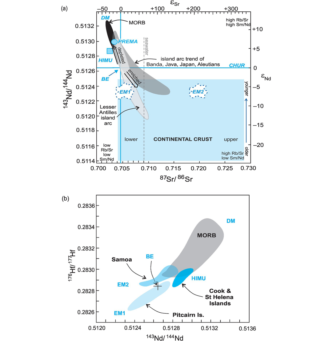
Mantle sources. (a) The 87Sr/86Sr versus 143Nd/144Nd diagram showing oceanic reservoirs for t = 0). These include the depleted mantle (DM), bulk silicate Earth (BE), enriched mantle (EM1, EM2), high-μ (U/Pb) (HIMU), and the ‘prevalent mantle’ (PREMA) compositions. The ‘depleted’ mantle reservoir in the upper left quadrant reflects residual mantle from which incompatible elements have been removed (it has been ‘depleted’). Most crustal rocks plot in the lower-right ‘enriched’ quadrant which includes old and young upper and lower crust. Mixing arrays between depleted mantle and enriched mantle sources are suggested by the island arc trends. Note the negative correlation between these two systems. Data compiled from Zindler and Hart (1986), Jackson et al. (2007) and White (2015). (b) The 143Nd/144Nd versus 176Hf/177Hf diagram of oceanic reservoirs with DM represented by global MORB, EM1 by volcanic rocks from the Pitcairn Islands, EM2 by volcanic rocks from the island of Samoa and HIMU by the Cook and St Helena Island volcanic rocks (after Stracke, 2016). The positive covariation on this diagram reflects the similar chemical behaviour of the parent/daughter elements in the two systems.
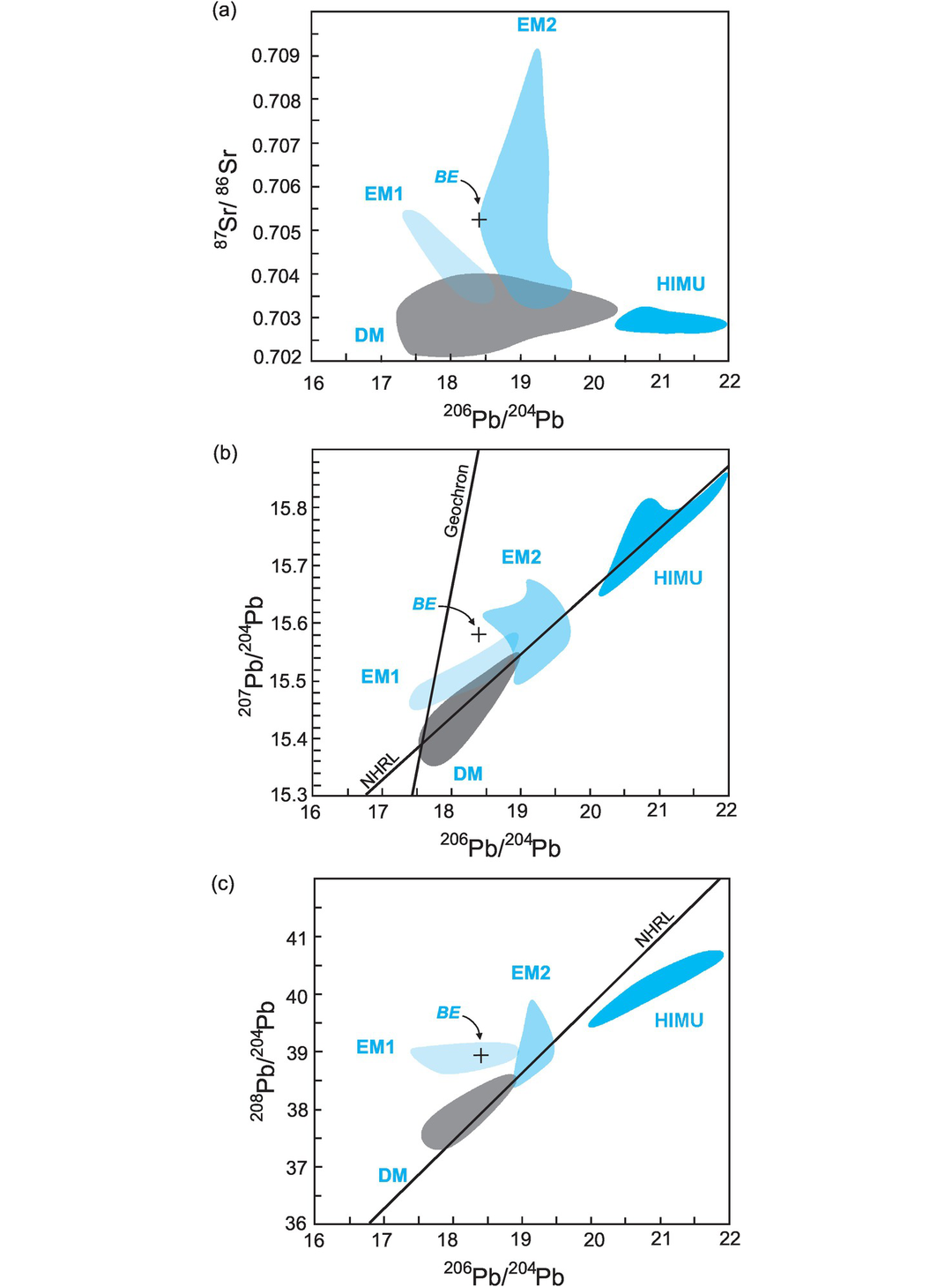
Mantle sources as defined by lead isotopes (data from Hofmann, 2014). (a) 206Pb/204Pb versus 87Sr/86Sr; (b) 206Pb/204Pb versus 207Pb/204Pb; (c) 206Pb/204Pb versus 208Pb/204Pb. Bulk silicate Earth (BE) is shown for reference (see Table 6.6 for values). The geochron assumes single-stage Pb-evolution from 4.55 Ga. NHRL is the Northern Hemisphere Reference Line (after Hart, 1984). Volcanic rocks which plot above the NHRL are said to have an enriched (DUPAL) signature. The non-controversial mantle reservoirs include the depleted mantle (DM) represented by global MORB, enriched mantle (EM1 by the Pitcairn Islands and EM2 by the island of Samoa), and high-μ mantle (HIMU) by the Cook and St Helena Islands. It is significant that the enriched mantle sources have some overlap with continental crustal sources (see Figure 6.10).
(b) The depleted mantle (DM) reservoir. The Earth’s depleted mantle is characterised by high Sm/Nd and low Rb/Sr element ratios. This leads to high 143Nd/144Nd and low 87Sr/86Sr isotope ratios. In addition, the DM has high 176Hf/177Hf and low 206Pb/204Pb. It is the primary source of most mid-ocean ridge basalts.
(c) The HIMU mantle reservoir. In lead isotope geochemistry the μ value is the ratio 238U/204Pb. The high 206Pb/204Pb, 207Pb/204Pb and 208Pb/204Pb observed in some ocean islands coupled with low 87Sr/86Sr (<0.7030) and intermediate 143Nd/144Nd and 176Hf/177Hf suggest a mantle source that is enriched in U and Th relative to Pb without an associated increase in Rb/Sr. This enrichment is thought to have taken place between 0.7 and 2.1 Ga (Hauri and Hart, 1993). A number of models have been proposed to explain the origin of this mantle reservoir. These include the mixing of altered oceanic crust (possibly contaminated with seawater) into the mantle via subduction, the loss of lead from this part of the mantle into the Earth’s core, and the removal of lead (and Rb) by metasomatic fluids in the mantle.
(d) Enriched mantle (EM) reservoirs. The enriched mantle has variable 87Sr/86Sr, low 143Nd/144Nd, low 176Hf/177Hf and high 207Pb/204Pb and 208Pb/204Pb for a given value of 206Pb/204Pb. Enriched mantle type 1 (EM1) has low 87Sr/86Sr, whereas enriched mantle type 2 (EM2) has high 87Sr/86Sr. Jackson et al. (2007) proposed an even higher 87Sr/86Sr (>0.702) for the EM2 component (as shown in Figure 6.10). A large-scale example of EM2 occurs in the Southern Hemisphere (Dupre and Allegre, 1983) and is known as the DUPAL anomaly (Hart, 1984). This component is identified with respect to a Northern Hemisphere Reference Line (NHRL) defined on plots of 206Pb/204Pb versus 207Pb/204Pb and 206Pb/204Pb versus 208Pb/204Pb by a linear array of mid-ocean ridge and ocean island basalts (Figure 6.11).
The equations for the NHRL in each of the plots is:
The isotopic anomaly was expressed by Hart (1984) in terms of Δ7/4 and Δ8/4, defined as the vertical deviation from the reference line, such that for a given data set (DS)
A similar notation was used for 87Sr/86Sr:
There are three models which are used to explain the origin of the enriched mantle. The first model is subduction-driven recycling, in which compositionally distinct components such as marine sediment, crustal sediment and upper and lower crust are recycled into the mantle via subduction. The second model is that of mantle metasomatism, that is, enriched by melts and fluids within the mantle (see Willbold and Stracke, 2010, for an overview). The third model is based upon the similarity between enriched mantle and the sub-continental lithosphere and suggests that the enrichment is due to the mixing of sub-continental lithosphere into the mantle. EM1 has some compositional similarity with the lower continental crust and may represent the mixing of recycled lower crust. Alternatively, it may be enriched via mantle metasomatism. EM2 has affinities with the upper continental crust and may represent the recycling of continentally derived sediment, continental crust, altered oceanic crust, or ocean island crust.
(e) Other reservoirs. In the 1980s and 1990s, as the field of mantle isotope geochemistry expanded, every ‘reservoir’ that was identified seemed unique. However, the mantle geochemical database has increased exponentially since that time and coupled with our improved understanding of melt extraction and mixing processes in the mantle we now define the number of compositional ‘end members’ or reservoirs as the minimum needed to explain the observed isotopic diversity. These are the DM, EM1, EM2 and HIMU end members. Other ‘components’, such as PREMA, PHEM, C and FOZO, represent compositional domains that may not be required, although this is the subject of ongoing discussion (see Hofmann, 2014, for an overview). Nonetheless, the reader may come across these terms in the literature and it is therefore useful to define them here.
PREMA (prevalent mantle) was defined by Zindler and Hart (1986) using basalts from ocean islands, intra-oceanic island arcs and continental basalt suites. It is characterised by 143Nd/144Nd = 0.5130, 87Sr/86Sr = 0.7033 and 206Pb/204Pb = 18.2–18.5.
PHEM (primitive helium mantle) was defined by Farley et al. (1992) using basalts mostly from the Samoan islands to account for their high 3He/4He, along with near-BE Sr and Nd compositions (87Sr/86Sr = 0.7042–0.7052, 143Nd/144Nd = 0.51265–0.51280) and moderately radiogenic Pb isotopes (206Pb/204Pb = 18.5–19.0).
FOZO (focal zone) was originally defined by Hart et al. (1992) as the region or zone in which MORB and OIB isotopic signatures seemed to converge (or focus, hence the term ‘focal zone’). Compositionally, it is similar to PREMA and C, although the term was later modified by Stracke et al. (2005) to extend the MORB array in 206Pb/204Pb (or 208Pb/206Pb) versus 87Sr/86Sr space. According to this later definition, the FOZO field identified in lavas from the Cook–Austral islands is adjacent to but distinct from HIMU in Pb isotope space.
C (common component). This component was defined by Hanan and Graham (1996), using the convergence of MORB Pb isotope arrays. It is very similar to FOZO, with 87Sr/86Sr = 0.703–0.704, 143Nd/144Nd = 0.51285–0.51295, 206Pb/204Pb = 19.2–19.8, 207Pb/204Pb = 15.55–15.65 and 208Pb/204Pb = 38.8–39.6.
(f) The origin of oceanic basalts. The recognition of a range of isotopic signatures in oceanic basalts associated with distinct mantle reservoirs has led to an appreciation of the complexity of mantle processes. This can be seen at the local scale, where, for example, detailed and high-precision isotopic studies of the Hawaiian–Emperor plume have identified multiple depleted and re-fertilised mantle components within a single plume (Béguelin et al., 2019; Harrison et al., 2020). At the global scale our perception of the mantle has changed from a simple two-layer mantle to one that is chemically and isotopically heterogeneous and contains at least four reservoirs. Sampling this heterogeneity is not trivial, for the process of partial melting homogenises those diverse compositions which have resulted from melt extraction, hybridization and mixing within the mantle.
6.3.2.2 Continental Crustal Sources
The isotopic composition of rocks from the continental crust is extremely variable, and isotope ratios are strictly comparable only if the samples are all of the same age. For this reason, compositional differences are best considered relative to a normalising parameter which takes into account the age of the sample. One such parameter is the composition of CHUR and its evolution through time; this is discussed in Section 6.3.3 below. Crustal samples may be plotted on a graph of isotopic composition versus time relative to reference reservoir (Figure 6.3). For Sr, Nd and Hf isotopes this can be quantified in terms of the epsilon notation, whereas Os isotopes use the gamma notation (these notations are discussed in Section 6.3.4). The general isotopic characteristics of crustal reservoirs are given in Table 6.6, and the isotopic compositions of some typical crustal rocks are presented in Table 6.7.
(a) Upper continental crust. The upper (sialic) continental crust is characterised by high Rb/Sr and consequently has high 87Sr/86Sr ratios. Neodymium and Hf isotope ratios, on the other hand, are low relative to mantle values as a consequence of the low Sm/Nd and Lu/Hf ratios which characterise the continental crust. U and Th are enriched in the upper continental crust and give rise to high 206Pb, 207Pb and 208Pb isotope ratios.
(b) Middle continental crust. The mid-continental crust represents extensive areas of exhumed amphibolite facies gneisses found in granite–gneiss terrains. These rocks have retarded 143Nd/144Nd and 176Hf/177Hf, and 87Sr/86Sr is generally lower than in the upper crust. Uranium, however, is depleted, and Th is lower than in the upper crust but not as depleted as U. 206Pb/204Pb and 207Pb/204Pb may be lower than in the mantle.
(c) Lower continental crust. The lower continental crust is characterised by mafic rocks and granulite facies metamorphosed rocks and is often strongly Rb-depleted. Thus, it has low 87Sr/86Sr ratios which are not greatly different from modern mantle values. This means that a modern granite derived from the lower crust will have an initial 87Sr/86Sr ratio very similar to one derived from the mantle. U/Pb and Th/Pb ratios in the lower crust are lower than modern mantle values so that 206Pb, 207Pb and 208Pb isotope ratios are all very low and are therefore sensitive indicators of lower crust and mantle reservoirs.
(d) Continental lithosphere. The continental lithosphere is the region of mantle that lies beneath and is attached to continental crust. In areas of ancient crust it is extremely thick. It is known as the continental lithospheric mantle (CLM) or the sub-continental lithospheric mantle (SCLM) and is extremely variable in isotopic composition. Isotope data from CLM-derived mantle xenoliths show that the CLM typically has higher 87Sr/86Sr (>0.7045), lower εNd (<0) and higher 207Pb/204Pb (at a given 206Pb/204Pb) when compared with asthenospheric mantle sources (Pearson, 1999). Nd and Hf isotopes are decoupled during the fractionation of the lithospheric mantle with the result that Nd isotopes are more readily reset than Hf isotopes during mantle metasomatism. Only very young (0.35 Ga) and small (<5%) depletion events can fractionate Lu from Hf, which results in 176Hf/177Hf compositions in the CLM similar to those in the present-day convecting mantle (εHf today ~ +11). Older and more extensive melting generally results in 176Hf/177Hf ratios that are more radiogenic than is seen in the convecting mantle and typically exceeds compositions recorded by mantle xenoliths. Os isotopic ratios in the CLM are in the range 187Os/188Os = 0.1100–0.1205 and are statistically distinct from peridotites from the convecting mantle (187Os/188Os = 0.1225–0.1265; Pearson and Wittig, 2014). This is illustrated in Figure 6.12.
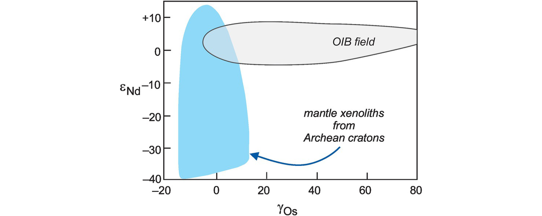
The isotopic composition of the continental lithospheric mantle (CLM) (after White, 2010; with permission from Elsevier). A γOs versus εNd diagram (see Section 6.3.4) showing the difference in composition between xenoliths from the CLM (mantle xenoliths from Archaean cratons in Siberia, Wyoming, and South Africa) and that of ocean island basalts (Cook–Austral islands, Hawai‘I and Samoa) representing the convecting mantle.
Most cratons are underlain by old CLM and the Re–Os isotope system is the preferred method for dating this ancient lithospheric mantle (Rudnick and Walker, 2009; Farmer, 2014). One of the best examples of the application of this method is from the Kaapvaal craton where the Mesoarchean craton was shown to be underlain by older, Eoarchean and Hadean lithospheric mantle which in turn is surrounded by lithospheric mantle reworked between 3.0 Ga and 2.0 Ga (Pearson and Wittig, 2014).
6.3.2.3 Seawater
A knowledge of the isotopic composition of seawater is important in studies of magmatic rocks which may have interacted with seawater such as the sea-floor alteration of oceanic basalts or the genesis of magmas in an arc environment, and in sediments such as the alteration rinds on sea-floor nodules. Its composition is related to the residence time of an element in seawater. This is the average time an element remains in seawater and is defined by the expression:
where tA is the residence time, A is the total amount of the element dissolved in the oceans, and dA/dt is the amount of the element introduced into or removed from the ocean per unit time assuming a steady state. It is estimated that the oceans mix over ~1000 years so that an element with a residence time longer than this will be homogeneously distributed in the ocean, whereas an element which has a shorter residence time will reflect regional variations in isotopic composition (see Frank, 2002, for an overview).
The residence time of Sr in seawater is a few million years and the oceans are regarded as a well-mixed reservoir with uniform 87Sr/86Sr = 0.70918 (Frank, 2002). This signature is the result of the solubility of Sr and the complex interplay between continental run-off, mid-ocean ridge hydrothermal activity, input from old sediments and the extraction of Sr into carbonate shells and their subsequent burial in marine sediments. Osmium has a shorter residence time, 10,000–20,000 years. Veizer et al. (1999) and Peucker-Ehrenbrink and Ravizza (2000) demonstrate how Sr and Os isotope compositions have changed in seawater over the past 60 million years (Figure 6.13). They showed that isotope ratios of both elements were relatively low in the late Cretaceous and have gradually increased with time, probably as a result of increased continental weathering related to the uplift of major mountain ranges. The seawater curves for Sr in the Phanerozoic, and particularly the high precision curve for the last 70 Ma, has been used to date sediments and to determine the time of diagenetic processes.
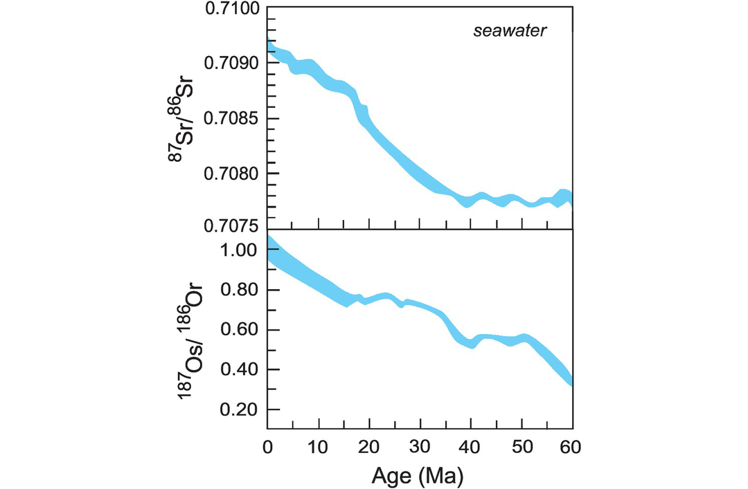
The isotopic variation in the composition of seawater over the last 60 Ma. The data for 87Sr/86Sr are from Veizer et al. (1999) and for 187Os/188Os from Peucker-Ehrenbrink and Ravizza (2000). The variation is thought to be associated with an increase in continental weathering during this time interval.
In contrast, Nd, Hf and Pb have shorter residence times: Nd 600–2000 years, Hf about 200 years, and Pb 50–400 years (Frank, 2002). These shorter residence times indicate that the oceans are not well mixed with respect to isotopes of Nd, Hf and Pb. In fact, it has been long known that the Nd isotopic composition of seawater (using the ε notation) ranges from εNd −27 to +1. This variability in 143Nd/144Nd between different ocean basins reflects the local Nd input from surrounding continents. The most radiogenic Nd isotopic compositions are found in the Arctic (εNd = −10.1), the least radiogenic in the Pacific (εNd = −3.9), and the Atlantic (εNd = −11.4) and Indian Oceans (εNd = −6.6) have intermediate compositions (Lacan et al., 2012). This pattern is also mirrored in the Hf and Pb compositions. 177Hf/176Hf in the Atlantic and Pacific Oceans ranges from εHf −5.7 to +8.6 (Rickli et al., 2014, and references therein). Manganese nodules concentrate Pb from seawater and have 206Pb/204Pb in the range 18.5–19.3 (von Blanckenburg et al., 1996).
6.3.3 Mantle Evolution Diagrams and the Isotopic Evolution of the Mantle with Time
The isotopic compositions of mantle source regions change with time as a function of their parent/daughter element ratios. These may be plotted on isotope evolution diagrams to show the change in isotopic composition of the reservoir with time. They are calculated by measuring the isotopic composition of the mantle at the present day using modern lavas and by determining initial ratios from isochron diagrams using samples of ancient mantle melts. Diagrams of this type are also useful for depicting the isotopic evolution of crustal rocks of different ages and with different parent–daughter isotope ratios. All evolution diagrams require a starting isotopic composition for the Earth at ~4.57 Ga, and as previously stated this is usually linked to the composition of meteorites (see Table 6.3).
The isotopic evolution of the mantle over geological time can be represented graphically in two different ways. One type of diagram shows the change in the isotope ratio from the beginning of the Earth to the present. This is illustrated for Nd isotopes in Figure 6.14a, which shows a linear increase in the 143Nd/144Nd ratio in the depleted mantle and in the chondrite reservoir with time. A second type of diagram uses the ε (epsilon) notation to display the isotopic composition relative to CHUR, the chondrite standard (Figure 6.14b). In this case CHUR has a value of zero and the ε value for the depleted mantle increases with time. A full discussion of the ε notation for Nd and Hf isotopes and its equivalent for Os isotopes – the γ notation – is given in Section 6.3.4.
6.3.3.1 The Evolution of Nd Isotopes with Time
The 143Nd/144Nd isotopic composition of the bulk Earth is thought to be approximated by the composition of chondritic meteorites (CHUR). The linear evolution of CHUR with time is shown in Figure 6.14a. However, studies of modern oceanic basalts, as well as ancient and modern granitic rocks, indicate that many igneous rocks are derived from a mantle composition which has a higher Sm/Nd than CHUR and has a higher 143Nd/144Nd ratio relative to CHUR – this is the depleted mantle (DM) reservoir. In Figure 6.14b three common models for the evolution of the depleted mantle reservoir are shown relative to CHUR using epsilon notation (see Section 6.3.4 and Box 6.2). The main differences between these models is the time at which the DM differentiated from the bulk Earth, and whether or not the depletion varied with time. Goldstein (1984) used a single-stage, linear evolution between the present day and the formation of the Earth at 4.6 Ga (Figure 6.14b, line 1), whereas DePaolo (1981a) used a non-linear model (Figure 6.14b, line 2).
Nägler and Kramers (1998) developed a 143Nd/144Nd evolution curve using mantle melts of known age free from crustal contamination and metamorphism (Figure 6.14b, line 3). They show that the average εNd for the early Archaean is fairly constant, whereas from about 3.0 Ga to the present, εNd steadily increases to a present-day value of +10. They conclude that the average εNd value for the early Archaean has no geological significance, being partly an analytical artefact and partly is the product of uncertainty in the measurement of Nd in chondrites. In contrast, the steady increase in εNd from 3 Ga to the present implies the progressive extraction of the LREE from the Earth’s mantle through the formation of the continental crust. The Sm/Nd of the continental crust is highly fractionated (<1.0) relative to CHUR and shows retarded 143Nd/144Nd evolution with time (Figure 6.14a).
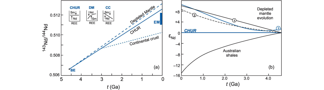
Evolution of Nd isotopes with time. (a) The evolution of 143Nd/144Nd for CHUR (solid line), DM (dashed line), and the continental crust (CC, dotted line) from the initial composition of the bulk Earth (BE). The fractionation of Sm/Nd from BE is normalised to unity for CHUR; DM has high Sm/Nd resulting in higher 143Nd/144Nd; and CC has lower Sm/Nd which retards 143Nd/144Nd evolution with time. The enriched mantle (EM) component (blue box) shows some affinity with the continental crust inasmuch as it also has retarded 143Nd/144Nd. Note that in the Sm–Nd system, the crust shows retarded isotopic evolution, whereas in the Rb–Sr system it shows accelerated evolution relative to BE and the mantle. (b) The contrasting evolution of the continental crust and mantle using εNd notation (Section 6.3.4). CHUR = 0 and plots as a horizontal line. Three curves are shown for the evolution of the depleted mantle. Line 1 assumes a single-stage, linear evolution for the depleted mantle between 4.5 Ga (εNd = 0) and the present day (εNd = +10) (Goldstein et al., 1984). Curve 2 assumes an exponential evolution that is derived from the equation 0.25t2 – 3t + 8.5, where t is the time before present in Ga (DePaolo, 1981a). Curve 3 is a multi-stage model that shows an inflection at ~3 Ga thought to reflect the initiation of the growth of the continental crust (Nägler and Kramers, 1998). The curve in the bottom half of the diagram is for Australian shales and approximates to the evolution of average continental crust through time (Allegre and Rousseau, 1984). Note the time axes in (a) and (b) are reversed.
(1) εNd values for an isochron
Using the data from Hamilton et al. (1979a) in Table 6.2, presented in Figure 6.2:
initial ratio = 0.50809
isochron age = 3.54 Ga
decay constant λ = 6.54 × 10⁻¹² yr−1
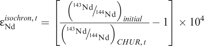
First calculate the value of CHUR at time t using the CHUR values from Table 6.4 (normalised to 146Nd/144Nd = 0.7219, Sm/Nd = 0.325):
CHUR, t = 0.512638 − (0.1967 × [e(6.54×10−12)×(3.54×10+9)−1])
= 0.512638 − 0.004607
= 0.508031
Then using Eq. 6.12:
εNdisochron, t = [(0.50809/0.508031)−1] × 104
= 1.16
(2) εNd value for a rock at its time of formation
Using a single rock from Table 6.2 (sample HSS-74, sodic porphyry, 147Sm/144Nd = 0.1030,
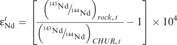
First, calculate 143Nd/144Nd rock at 3.54 Ga:
εNdt = 0.510487 − (0.1030 × [e(6.54×10−12)×(3.54×10+9)−1])
= 0.510487 − 0.002412
= 0.508075
Then from Eq. 6.14:
εNdt = [(0.50807/0.512638) − 1] × 104
= 0.87
(3) εNd value for a rock at the present day
The present-day deviation from CHUR may be easily calculated from:
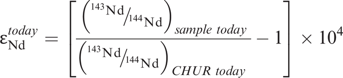
Summary
6.3.3.2 The Evolution of Hf Isotopes
During mantle melting the fractionation of Lu relative to Hf is more extreme than for Sm and Nd. This generates a more strongly supra-chondritic εHf signature than seen in εNd for the same melting event. This is documented in modern oceanic basalts where εHf is up to 1.5 times greater than εNd (Vervoort and Blichert-Toft, 1999). Söderlund et al. (2004) proposed a single-stage evolution line for 176Hf/177Hf in the mantle (expressed as εHf in Figure 6.15a) from ~4.6 Ga. This model is consistent with the work of Kemp et al. (2010), who showed from Hf isotopes in zircon that there was a depleted mantle in the Hadean. However, some authors have argued for a supra-chondritic mantle in the early Earth (Caro and Bourdon, 2010; Kemp and Hawkesworth, 2014).
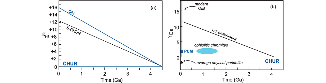
Mantle evolution with time for Hf and Os isotopes. (a) Hafnium isotopes (using εHf notation) showing two linear models for mantle evolution for εHf in the depleted mantle (DM) (after Söderlund et al., 2004) and for S-CHUR (after Caro and Bourdon, 2010). (b) Osmium isotopes (using γ notation) showing Os enrichment of the mantle as a function of time. Note the wide range of modern OIB compositions and the near-chondritic nature of some ophiolitic chromites; the primitive upper mantle (PUM), CHUR and average abyssal peridotite are shown for reference.
6.3.3.3 The Evolution of Os Isotopes
Re is a moderately incompatible element during partial melting and so enters the melt phase, whereas Os is strongly compatible and remains in the unmelted residue. This leads to high Re/Os ratios in oceanic crust and relatively low Re/Os ratios in the depleted mantle. In felsic melts, however, Re and Os are both incompatible, and their concentrations are very low in the continental crust. This is very different from the Nd, Hf and Pb isotopic systems. These geochemical properties mean that the Os isotopic evolution of the upper mantle reflects the extraction of basaltic melts and is unlikely to reflect any interaction with the continental crust. Mantle melts which have supra-chondritic Os isotopic ratios are thought to be derived by the melting of ancient, high Re/Os, basaltic crust which has been recycled back into the mantle, making Os isotopes important ‘tracers’ of recycled ancient oceanic crust.
Figure 6.15b shows that OIB defines a wide range of 187Os/188Os ratios. This can be due to seawater contamination and/or the rapid in-growth of radiogenic 187Os in melts which have a high initial Re contents. This ‘Os enrichment’ trend is seen in mantle plume–related samples, whereas some ophiolitic chromites have near-chondritic Os signatures (Figure 6.15b). Both the chondritic and the enriched ‘reservoirs’ must be long-lived features of the mantle since the parent isotopes require a long period of time to evolve into the isotope ratios measured today.
6.3.3.4 The Evolution of Pb Isotopes
The isotopic evolution of lead isotopes over geological time is illustrated in Figures 6.16 and 6.17. Given that there are three independent decay schemes in the lead isotopic system, Pb data is not displayed on the same type of time versus isotope ratio diagram as is used for Sr, Nd, Hf and Os isotopes; rather, a concordia diagram is used. On this diagram ‘families’ of concordia (growth) curves can be drawn for different 238U/204Pb (μ values) (Figure 6.16a, b). Each curve can be calibrated for time, and equal time points can be used to generate isochrons (Figure 6.16b, c). Bolhar et al. (2020) used this approach to calculate a Pb isochron age of 2054 ± 99 Ma for phoscorites and carbonatites from the Phalaborwa Complex, South Africa. These authors then used the isochron age to evaluate the relative crust and mantle contributions to the sulphide genesis.
The evolution of Pb isotopes in the mantle through time is shown in Figure 6.17 on a plot of 206Pb/204Pb versus 207Pb/204Pb (after Kramers and Tolstikhin, 1997). This figure illustrates the evolution of Pb isotopes over time from a chondritic starting composition of the early Earth. It is clear that there is a wider range of 207Pb/204Pb than 206Pb/204Pb in early Earth history and wider range of 206Pb/204Pb relative to 207Pb/204Pb during the more recent evolution of the Earth. This diagram also shows that a HIMU mantle evolves with a lower 207Pb/204Pb than that of the depleted mantle (Kamber, 2015).
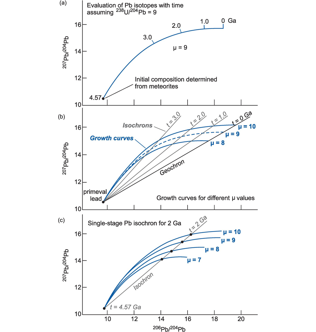
Lead isotope evolution curves. All panels show the growth curve(s) for 207Pb/204Pb and 206Pb/204Pb through time. (a) The isotopic evolution of 207Pb/204Pb and 206Pb/204Pb defines a curve because the two isotope ratios are produced at different rates. The starting composition at 4.57 Ga is taken from the isotopic composition of troilite in the Canyon Diablo meteorite (Box 6.1). This growth curve assumes a 238U/204Pb ratio (μ value) = 9.0. (b) A family of growth curves showing lead isotope growth associated with different 238U/204Pb ratios (μ = 8, 9 and 10), from primeval Pb at 4.57 Ga to the present. Isochrons for 0, 1.0, 2.0 and 3.0 Ga are created by joining similar age points on each growth curve. The zero Ga isochron is known as the geochron (see Section 6.2.1.4). (c) A single-stage lead isochron for 2.0 Ga. The isochron joins the 2.0 Ga points on the growth curves for four different μ values and passes through the primeval lead composition at 4.57 Ga; it represents a suite of samples which evolved from 4.57 Ga until 2.0 Ga. These values have remained ‘frozen’ in the samples since 2.0 Ga. The growth curves in these diagrams are based upon the assumption that the lead isotopes have evolved uninterrupted since the formation of the Earth. This is a simplification; normally a more complex model of lead isotope evolution is adopted, such as that of Stacey and Kramers (1975) or Kramers and Tolstikhin (1997).
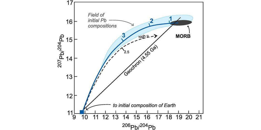
The evolution of lead isotopes with time. A 206Pb/204Pb versus 207Pb/204Pb plot showing the evolution of the depleted mantle (blue curve; after Kramers and Tolstikhin, 1997) and a HIMU mantle source (dashed curve; after Kamber, 2015). Note that the HIMU source has lower 207Pb/204Pb than DM for young samples. The MORB field and the field of initial Pb composition for crustal and mantle rocks are indicated. The numbers on the isotope evolution curves represent the time before the present in Ga.
6.3.4 Epsilon, Gamma and Mu Notations
Isotope ratios are only strictly comparable if the samples are of the same age. It is therefore useful to have an alternative way of expressing isotope ratios which allows greater flexibility in the way in which they are represented and is independent of their age. This is the basis of the ε notation used in the Nd, Hf and Sr systems (DePaolo and Wasserburg, 1976) and the γ notation used for Os isotopes (Walker et al., 1989).
6.3.4.1 Calculating Epsilon Values
The epsilon parameter is a measure of the difference between an isotope ratio from a sample or a suite of samples such as 143Nd/144Nd or 176Hf/177Hf, and a reference value, typically CHUR. It is expressed in parts per 104 (see worked example in Box 6.2). Epsilon values are used in three slightly different ways, as described below.
(a) Epsilon values calculated for an isochron. The epsilon value for an isochron is calculated using the expression:
where (143Nd/144Nd)initial is the measured initial ratio of the sample suite at the time of its formation (t) and is calculated from the isochron. (143Nd/144Nd)CHUR,t is the isotope ratio of CHUR at time (t) given by the expression:
where λ is the decay constant of 147Sm to 143Nd and t is the time of interest. Values for CHUR are given in Table 6.3. It should be noted that different laboratories use different normalising values for 143Nd/144Nd and a consistent value of CHUR must be selected. However, if this is done, then any variation in 143Nd/144Nd due to interlaboratory differences virtually disappears, making the epsilon notation a very useful way of displaying data generated in different laboratories.
The equations for the Hf system are similar:
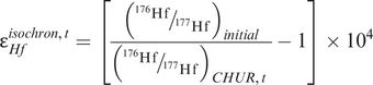
where (176Hf/177Hf)initial is the measured initial ratio of the sample suite at the time of its formation (t) and is calculated from the isochron. (176Hf/177Hf)CHUR,t is the isotope ratio of CHUR at time (t) and is given by the expression:
where λ is the decay constant of 176Lu to 177Hf and t is time in the past for the part of the evolution curve of interest. Values for CHUR are given in Table 6.3.
(b) Epsilon values for individual samples at their time of formation. The epsilon value for an individual rock sample calculated for time t, the time of formation, is usually tabulated along with Sm–Nd and Lu–Hf isotopic data. It is calculated using the expressions:
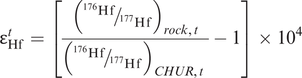
where the composition of CHUR at time t is calculated from Eq. 6.15 or Eq. 6.17. When calculating εNdt for individual samples the value for t may be taken either from the isochron to which the samples belong or from an independent estimate of the age using some other geochronological technique such as a U–Pb zircon age.
(c) Epsilon values for individual samples at the present day. An epsilon value may also be calculated for an individual sample at the present day using the expression:
The magnitude of the present-day εNd value reflects the degree of time-integrated depletion in Nd relative to CHUR, as expressed by the Sm/Nd ratio (see fSm/Nd, Section 6.3.4.6). Again, such calculations are equally relevant to the Lu–Hf system and may occasionally be applied to the Rb–Sr system.
6.3.4.2 Epsilon Values for Sr Isotopes
Epsilon values may be calculated from 87Sr/86Sr ratios in exactly the same way as for Nd isotopes. Original estimates for the 87Sr/86Sr composition of the bulk Earth as a reference value vary significantly, but Salters and Stracke (2004) define a well-constrained BE composition of 0.7045 (Table 6.3). Using a realistic trace element ratio (Rb/Sr = 0.29–0.30) and assuming an initial 87Sr/86Sr of 0.69898, their BE composition yields 87Sr/86Sr values which are in agreement with values for modern MORB.
6.3.4.3 Calculating Gamma Values for Os Isotopes
The bulk Earth has near-chondritic 187Os/188Os and any deviations are relatively small, so a percentage variation from CHUR is easily expressed using the expression:
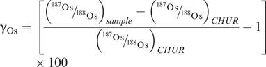
The ‘gamma’ parameter is directly analogous to the epsilon notation, but uses percentage of deviation instead of parts per 104. Here we term the reference material as CHUR; other workers use the term ‘CHON’. The two are interchangeable and reference values are given in Table 6.3a.
6.3.4.4 Reducing Epsilon Uncertainties on Isochron Diagrams
Points on a Sm–Nd isochron typically plot far from the origin. In order to obtain a greater degree of accuracy in determining the initial ratio, it is possible to plot felsic rocks (with small Sm/Nd ratios) on the same isochron as basic igneous rocks with larger Sm/Nd ratios if they are cogenetic. As cogenicity is not always established, an alternative method for reducing the error associated with calculating initial ratios, and hence epsilon values, is to translate the origin of the 147Sm/144Nd axis from zero to the present-day composition of CHUR (0.1960; Table 6.3) before performing the line-fitting operation (Fletcher and Rosman, 1982). With this translation the 147Sm/144Nd origin usually falls within the compositional range of the data set and results in a more precise determination of the intercept. This intercept value is the present-day composition of 143Nd/144Nd in a hypothetical sample which has the same 147Sm/144Nd as CHUR. This value may then be compared with CHUR to calculate the epsilon value using the equation:
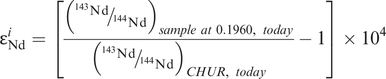
The definition of εiNd differs from εisochron,tNd (Eq. 6.14), but the difference between the two calculated values in terrestrial rocks is less than 1%, or less than 0.1 epsilon unit.
6.3.4.5 The Significance of Epsilon Values
εtNd is the ‘initial’ value of εNd in a sample at the time of its crystallisation and is useful because it provides information about the magma source. For example, if an isochron calculation yields εtNd = 0, the epsilon value indicates that the magma was derived from a mantle reservoir which had a chondritic Sm/Nd from the origin of the Earth until time t. A positive epsilon value for igneous rocks implies a magma derived from a source with a greater Sm/Nd than CHUR, that is, a depleted mantle reservoir. A negative epsilon value implies a source with a lower Sm/Nd than CHUR, that is, an enriched mantle or crustal source. Epsilon values for individual samples may be calculated as a test of cogenicity of samples used in an isochron plot.
Epsilon values (today) for individual samples are a measure of the extent to which the samples are fractionated relative to CHUR, as defined by the fractionation factor fSm/Nd (Section 6.3.4.6). Epsilon values vary with time and the following approximation may be used to calculate epsilon for some time (t) in the past from epsilon measured (today):
where fSm/Nd is given by Eq. 6.24 and Q = 25.13 Ga−1 when 146Nd/142Nd is normalised to 0.63151 (DePaolo, 1988) or Q = 25.09 Ga−1 when 146Nd/144Nd is normalised to 0.7219.
6.3.4.6 The Fractionation Factor fSm/Nd
The fractionation factor (f) is the 147Sm/144Nd analogue of epsilon and it is a measure of Sm/Nd enrichment in a given reservoir relative to CHUR. It is often written as fSm/Nd and is calculated from the expression:
Thus, an fSm/Nd value of +0.09, as is adopted for one model of the DM, has a time-averaged Sm/Nd which is 9% higher than CHUR. Over time this leads to positive εNd values for the depleted mantle. 3.8 Ga metakomatiites from Labrador have εNd values between +0.16 and +0.59, indicating a depleted mantle source with a substantially higher Sm/Nd than CHUR (Collerson et al., 1991). This is illustrated in Figure 6.18 and shows how samples with high positive fSm/Nd values evolve to very high present-day εNd values.
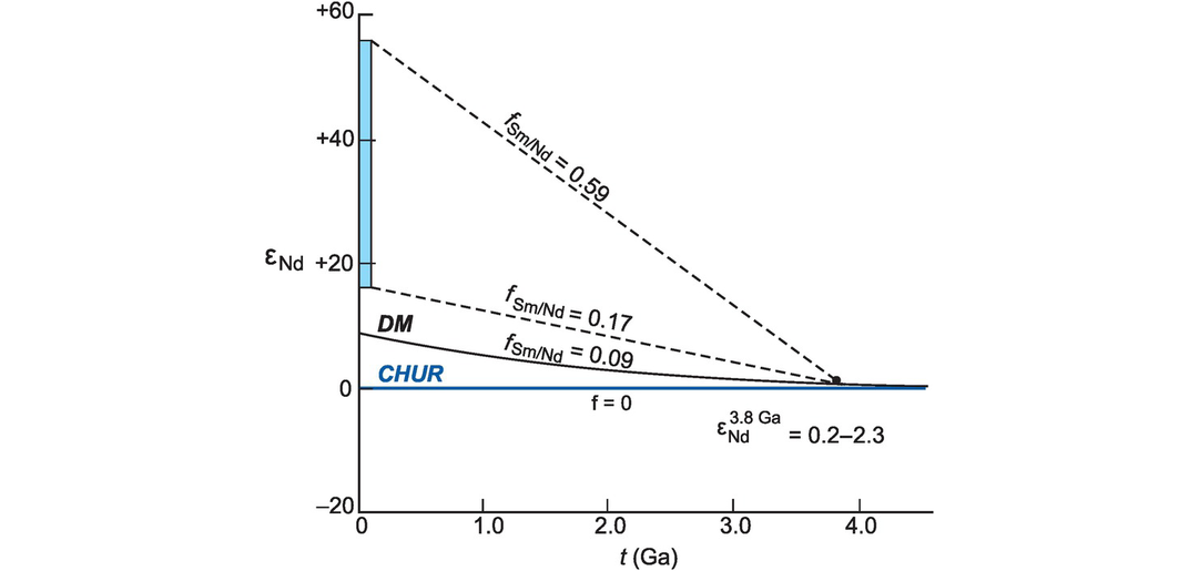
The variation of fSm/Nd with time. Epsilon evolution diagram using variable Sm/Nd ratios (fSm/Nd). This example is for 3.8 Ga meta-komatiites from Labrador (after Collerson et al., 1991). The komatiites were produced from depleted mantle at 3.8 Ga with individual εNd for the samples ranging from = +0.2 to +2.3, and with fSm/Nd varying from 0.17 to 0.59. Individual samples have evolved to present-day epsilon values of +16 to +56. The metakomatiites show extreme depletion relative to the depleted mantle (DM, fSm/Nd = 0.09) of DePaolo (1981a).
6.3.4.7 Epsilon Nd Time Plots
A convenient way of plotting calculated εNd values and eliminating inter-laboratory differences associated with generating 143Nd/144Nd is an epsilon–time evolution diagram. This is analogous to the mantle evolution diagram described in Section 6.3.3 and shown in Figure 6.14. Many workers plot εNd relative to CHUR and a model DM as a means of determining the likely mantle source of the sample (Figure 6.9). εNd calculated for individual samples may also be plotted, provided the age of the sample is known. In addition, individual sample evolution curves may be drawn for different values of fSm/Nd (Figure 6.18).
In contrast to DM, the continental crust shows retarded 143Nd/144Nd evolution with time relative to CHUR and generally has negative εNd values (Figure 6.14). The curve for Australian shales (Figure 6.14b) is thought to approximate the evolution of average continental crust through time (Allegre and Rousseau, 1984).
6.3.4.8 Short-Lived Isotopes and the μ Notation
(a) The 146Sm-142Nd system. 142Nd is a short-lived isotope produced by the decay of 146Sm with a half-life of 103 Ma. This means that 142Nd was produced only during the first few hundred million years of Earth history. Today 146Sm is extinct and 142Nd is no longer produced. Evidence of 146Sm → 142Nd decay is recorded as a 142Nd anomaly and these are found only in ancient rocks where they are an indicator of processes which took place during the Hadean – a time interval that is opaque to many other isotopic methods. Modern mantle rocks do not have 142Nd ‘anomalies’, indicating that the anomalies have been erased over geological time.
A 142Nd anomaly represents the deviation of the measured isotopic composition from that of a standard and is expressed in ppm. The standard currently in use is the synthetic standard JNdi-1 which represents the average 142Nd/144Nd ratio in the Earth today. Deviations from the standard are represented by the symbol μ (mu), which is defined in a manner analogous to that of εNd:
μ142Nd values may be recorded as excesses or deficits (positive or negative anomalies) indicating an incompatible element–depleted mantle reservoir or an enriched crustal reservoir, respectively.
142Nd anomalies tell us that the rock sample was originally extracted from a mantle domain in which 146Sm was ‘live’, and so within the first 300 Ma of Earth history. Rizo et al. (2011) report lavas from the 3.7–3.8 Ga Isua Greenstone Belt in west Greenland which record 142Nd excesses relative to the terrestrial standard (Figure 6.19), indicating that they were derived from a mantle source which was depleted in incompatible elements within the first 300 Ma of Earth history. Mafic rocks formed at 3.3 Ga from the same area of Greenland do not show 142Nd anomalies, indicating that by 3.3 Ga the mantle in this region had been homogenised (Rizo et al., 2013; Figure 6.19). Rizo et al. (2011) also found that once the 142Nd signature is preserved in ancient magmatic rocks, it is not modified by post-magmatic processes, leading them to conclude that ‘after 147Sm became extinct (at ca 4.2 Ga) no geological process is capable of generating 142Nd variations’.
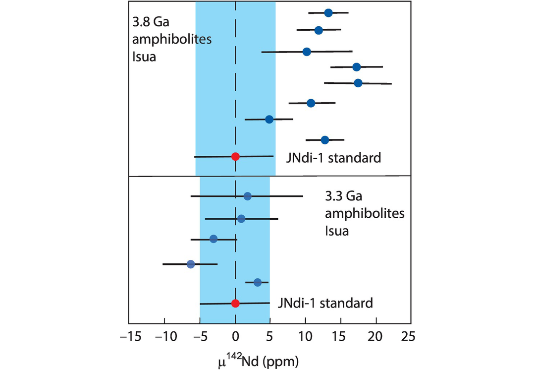
Variations in μ142Nd. Variations in μ142Nd in rocks from Isua in west Greenland. Sample compositions are plotted relative to the terrestrial JNdi-1 standard shown as the blue shaded area. 3.8 Ga amphibolites show positive deviations in μ142Nd, indicating their derivation from a depleted mantle source in the Hadean; 3.3 Ga amphibolites show no deviation from the terrestrial standard, indicating that by this time all 142Nd was homogenised in the mantle.
(b) The 182Hf–182W system. The 182Hf → 182W system has a half-life of 8.9 Ma and so is valuable for measuring events in the first 50 Ma in the solar system. This isotope system is important in understanding metal-silicate differentiation processes since W is moderately siderophile and Hf is strongly lithophile; it has been used to estimate the time of core formation (Schoenberg et al., 2002). In silicate systems W is more incompatible than Hf, and so variations in Hf/W can also result from the processes of crystal–liquid fractionation. Tungsten isotopes are measured as the 182W/184W isotope ratio and deviations from the Alfa Aesar standard are represented as μ values analogous to μ142Nd; μ182W is expressed in ppm (Rizo et al., 2016).
6.3.5 Isotope Correlation Diagrams
Given the contrasting behaviour of the different isotopic systems outlined in Section 6.3.1, it is instructive to investigate more than one isotope system in given a suite of rocks. This allows us to identify correlations between pairs of isotope ratios, which in turn lead to a better understanding of their petrogenesis. The simplest way to investigate relationships of this type is on an isotope correlation diagram: an x–y graph on which a pair of isotope ratios is plotted. Diagrams of this type are used to display the contrasting compositions of crust and mantle reservoirs (Figures 6.10 and 6.11) and are a means of investigating mixing processes between sources of contrasting composition.
It is, however, unlikely that petrogenetic processes can always be satisfactorily reduced to two dimensions, and Hart et al. (1992) proposed a three-dimensional projection of Sr–Nd–Pb isotopes for oceanic basalts. This plot (Figure 6.20) better illustrates the controls on the Sr–Nd–Pb systematics of oceanic basalts by showing the influence of specific components. For example, the relative contributions of EM1 in samples from the Pitcairn Islands and EM2 in samples from Samoa is notable.
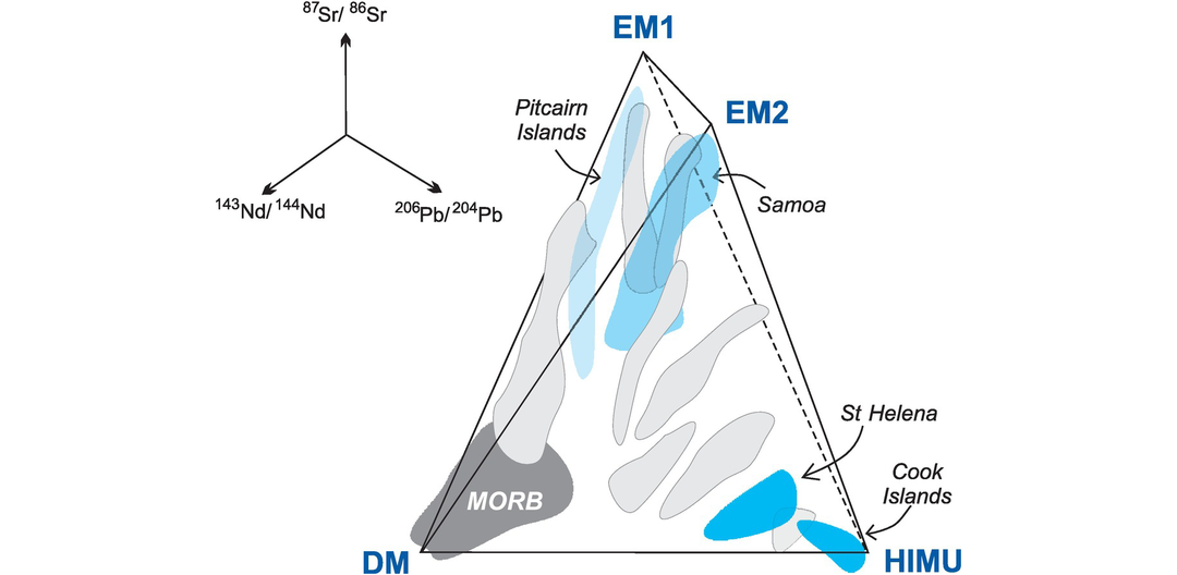
Three-dimensional projection of Sr, Nd and Pb isotopes for oceanic basalts. The interrelationship of the four principal mantle reservoirs is shown in this three-dimensional projection of Sr, Nd and Pb isotopes for oceanic basalts (data from Hart et al., 1992). Coherent trends between reservoirs indicate relative contributions of specific sources to particular OIB systems. For example, the compositional field of the Pitcairn Islands samples extends towards the EM1 component, whereas samples from Samoa trend towards EM2.
6.3.5.1 Using Isotope Correlation Diagrams and Epsilon Plots to Recognise Processes
Trends on isotope correlation diagrams are most commonly interpreted as mixing lines or mixing arrays. The ‘mixing’ may occur in the source region, during melt migration or in a magma chamber. Mixing in the source region may involve melts from different mantle reservoirs or melts produced by different degrees of partial melting. Mixing during melt migration may reflect melt–rock reaction in either the mantle or the continental crust, and, similarly, mixing in a magma chamber may be the result of reaction between the magma and the wall rock of the magma chamber or through the influx of compositionally distinct melts. There is software to model petrological mixing processes (see Chapter 4, Section 4.2.2), although a simple mixing equation such as that described by Langmuir et al. (1978) can easily be applied to isotope ratios. Compositions that result from mixing normally lie on a hyperbolic curve (see also Section 4.8.2), although if the ratios have a common denominator, as in the case of 87Rb/86Sr versus 87Sr/86Sr or 206Pb/204Pb versus 207Pb/204Pb, then mixing will produce a linear trend. This straightforward approach can determine whether or not a hypothesis is viable and may place constraints on end-member compositions, distinguish between the mixing of sources and the mixing of magmas, and even determine whether mixing is recent or ancient.
(a) Mixing between sources. For a number of years students of basalt chemistry have regarded the isotopic compositions of oceanic basalts as the result of mixing of different mantle sources. This is suggested by the linear and curvilinear arrays on isotope correlation diagrams such as the Sr–Nd mantle array (Figure 6.10) and the Pb–Pb isotope NHRL (Figure 6.11). Similar principles apply to mixing between crust and mantle sources, and we illustrate this process in Figure 6.21 with a Nd–Sr isotope correlation diagram (after DePaolo and Wasserburg, 1979) for rear-arc basalts from the Southern Volcanic Zone (SVZ) of the Chilean Andes (data from Turner et al., 2017). The authors show that there is a mismatch between the isotopic composition of the volcanic rocks and a DM–SVZ sediment mixing line; instead, the data define a mixing line between DM and EM1, suggesting their derivation from mixing between the DM and the continental lithospheric mantle.
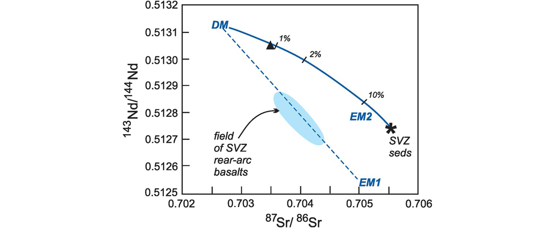
Sr–Nd isotope mixing diagram. 87Sr/86Sr versus 143Nd/144Nd (data from Turner et al., 2017) showing the theoretical (hyperbolic) mixing trend between DM and sediment of the Southern Volcanic Zone (SVZ), Chile (asterisk). The percentages indicate the amount of sediment mixed. EM2 and altered oceanic crust (triangle) are shown for reference. SVZ rear-arc basalts do not lie on this mixing trend but instead lie on a line between DM and EM1. Turner et al. (2017) use these relationships to argue that mixing between DM and SVZ sediment (or EM2) cannot explain the data trend, and therefore an EM1-like component is needed. Combining this with trace element data, the authors suggest that this component represents a metasomatised continental lithospheric mantle.
Mixing within the mantle and between the crust and mantle inevitably leads to deeper questions about mechanisms and scales of mixing and how these relate to plate tectonic processes. This takes us into the field of geodynamics, which we return to in Section 6.3.6.
(b) Mixing in a magma chamber. Layered mafic intrusions provide an opportunity to examine magma chamber processes and the process of crustal contamination. Wilson et al. (2017) analysed more than 130 samples from 2000 metres of drill core from the lower Bushveld series in South Africa. They used in situ LA-MC-ICPMS microanalysis of plagioclase crystals from the Lower Zone, the Marginal Zone, and the Basal Ultramafic Sequence (upper and lower) to document variations in the 87Sr/86Sri(2055 Ma) ratio between 0.7045 and 0.7073 (Figure 6.22). In detail, this profile shows small-scale, cyclic variations superimposed on larger-scale variations, which they attribute to sharp decreases in 87Sr/86Sri reflecting mixing between the resident magma and the influx of a more primitive magma.
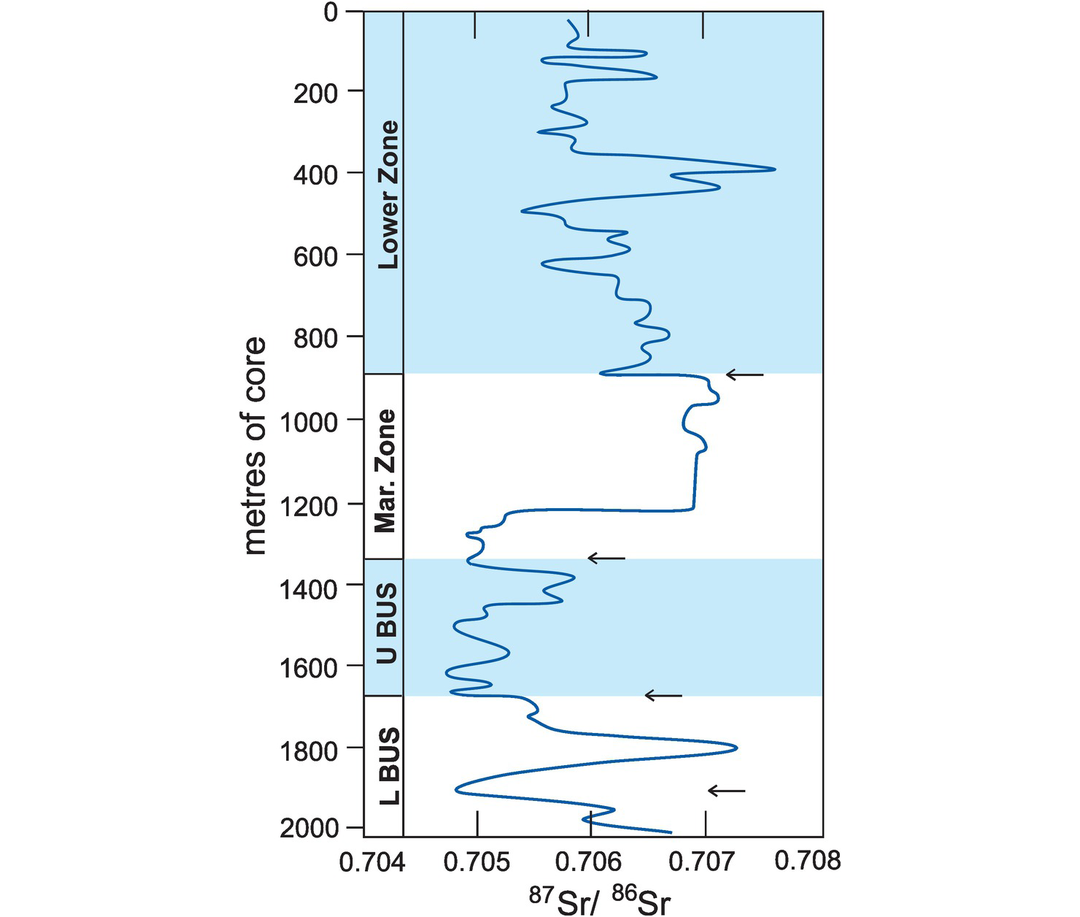
Mixing in a magma chamber. Variable 87Sr/86Sri(2055 Ma) within the lower series of the Bushveld intrusion, South Africa (data from Wilson et al., 2017). Compare the small-scale variations within the upper basal ultramafic sequence (U BUS) or the higher part of the marginal (Mar.) zone, with the large-scale variations between them. Arrows denote sharp decreases in 87Sr/86Sri ratios interpreted to reflect influx of more primitive melt.
6.3.5.2 Crustal Contamination
The phrase ‘crustal contamination’ is normally used to describe mantle melts which have interacted with continental crust. However, it is also used to describe a mantle source region into which crustal material has been introduced at some time in the past by a process such as sediment subduction. It is important to try to distinguish between these two possibilities.
(a) Magmatic contamination by continental crust. Pb is the most sensitive of the radiogenic isotopes to crustal contamination; Sr is moderately sensitive; and Nd is the least sensitive, although the combined application of radiogenic isotopes, stable isotopes (Section 7.3.1.3) and trace element ratios (Section 4.6) provides the best means of understanding the process of crustal contamination.
One helpful approach to quantifying crustal contamination is to study continental flood basalts on the basis that mantle-derived melts are sensitive to contamination from the continental crust and that the rapid emplacement of large volumes of basalt over short periods of time limits the interaction between them such that both components can be recognised. Haase et al. (2019) applied this approach to the Deccan flood basalts in India (Figure 6.23). They assumed that the parental magma was similar to a Réunion basalt but identified two additional components involved in the genesis of the Deccan magmatism. These were a crustal component with high 206Pb/204Pb, high 87Sr/86Sri and low εNd, which they interpreted as Archaean felsic lower crust, and a crustal component with low 206Pb/204Pb, intermediate 87Sr/86Sri, and highly negative εNd representing a feldspar-rich contaminant. By combining this information with incompatible trace element ratios they proposed a two-stage evolution for the Deccan magmatism in which a parental magma first stagnates in the Archean lower crust and subsequently mixes with a plagioclase-rich crustal component.
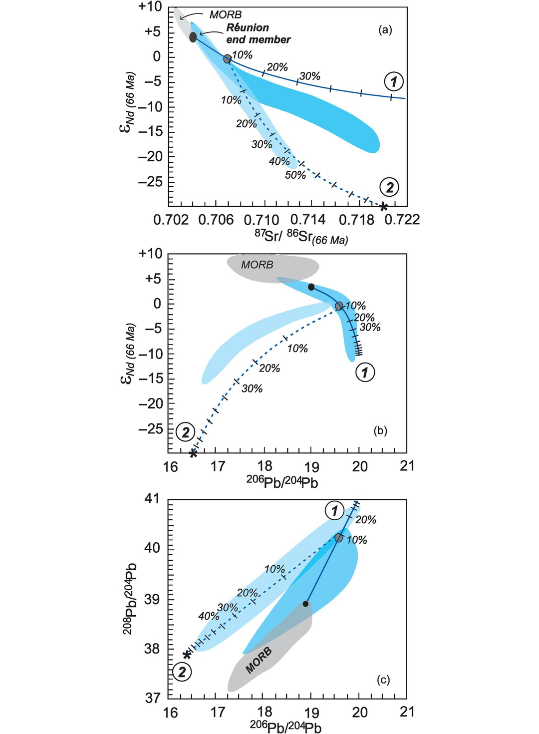
Crustal contamination of Deccan basalts. (a) 87Sr/86Sri (66 Ma) versus εNd; (b) 206Pb/204Pb versus εNd; and (c) 206Pb/204Pb versus 208Pb/204Pb. Deccan flood basalts have Sr, Nd and Pb isotopic compositions that define two compositional trends, implying a three-component mixing scenario (after Haase et al., 2019). The end-member compositions include a parental Réunion basalt (black dot), crustal component 1 (high 206Pb/204Pb, high 87Sr/86Sri and low εNd), and crustal component 2 indicated by the asterisk (low 206Pb/204Pb, moderate 87Sr/86Sri and highly negative εNd). Stage 1 involves the Réunion parent melt assimilating ~10% of crustal contaminant 1 and producing a hybrid melt (grey dot); this leads to stage 2, when the hybrid melt assimilates up to 50% of a plagioclase-rich crustal component.
(b) Crustal contamination and AFC processes. DePaolo (1981b) has shown that assimilation and fractional crystallisation (AFC) may shift compositions on an isotope correlation diagram far from what might be expected on the basis of simple mixing. On an Nd–Sr isotope correlation diagram simple mixtures will define a straight-line trend between the magma and contaminant, whereas in AFC processes when the bulk solid/liquid distribution coefficients for Nd and Sr differ markedly, then there is a significant departure from the simple mixing curve. A full discussion of AFC process is given in Section 4.2.2.3.
(c) Contamination with seawater. The isotopic composition of seawater is highly variable (Figure 6.3). Modern seawater has a high 87Sr/86Sr ratio (>0.709) relative to the mantle values of MORB (Farrell et al., 1995) and a moderate concentration of Sr, so the exchange of Sr between seawater and oceanic crust will produce relatively radiogenic 87Sr/86Sr ratios in young MORB. The 187Os/188Os ratio of modern seawater is ~1.1 (Woodhouse et al., 1999), which is 10 times higher than the mantle value, and the precipitation of Fe- and Mn-oxyhydroxides on submarine lavas concentrates seawater Os on the surfaces of sea-floor rocks and increases the 187Os/188Os ratio. In contrast, the elements Nd and Hf are relatively insoluble in seawater, and so isotope ratios tend to be insensitive to seawater contamination: 143Nd/143Nd in seawater is low (εNd = −1 to −18), whereas 177Hf/176Hf is intermediate (εNd = +8 to −4) (Rickli et al., 2009; Stichel et al., 2012). Consequently, on a 87Sr/86Sr versus 143Nd/144Nd diagram the effect of contamination by seawater will show enhanced 87Sr/86Sr at relatively constant 143Nd/144Nd. Pb isotopes in seawater vary widely (206Pb/204Pb = 17.25 – 19.75, 207Pb/204Pb = 15.3 – 15.65, 208Pb/204Pb = 37 – 39.8) and are susceptible to anthropogenic contamination.
6.3.5.3 Isotope versus Element Plots
Since an isotope ratio cannot be fractionated by crystal–liquid equilibria and is therefore indicative of the magmatic source, the correlation between an isotope ratio and a major or trace element can be used as a guide to the major element or trace element composition of the source. Typically, ratios of highly incompatible trace elements (Section 4.6.1 and Table 4.11) are the most useful for characterising the elemental composition of the source region. Thus, correlations between isotope ratios and ratios of highly incompatible trace elements are likely to indicate mixing between compositionally distinct sources.
Figure 6.24 shows the strontium isotope ratio plotted against Nb/U for basalts from the Society Islands (an EM2 source). Nb and U are highly incompatible elements but have similar bulk partition coefficients during mantle melting in most oceanic environments. Consequently, the limited Nb/U ratio in oceanic basalts should reflect the composition of their source. As the two axes do not share a common denominator, mixing in this diagram should define a curve rather than a straight line (Langmuir et al., 1978). Oceanic rocks (MORB and non-EM-OIB) have a Nb/U ratio of ~36–67 (Hofmann, 2014) and continental crust a ratio of Nb/U = 8 (Rudnick and Fountain, 1995); sediment has consistently higher 87Sr/86Sr ratios than MORB and OIB. Thus, OIB containing significant amounts of recycled sediment should be distinguished by high 87Sr/86Sr and low Nb/U ratios, and the observed trend towards high 87Sr/86Sr and low Nb/U is consistent with mixing between mantle and continental crust.
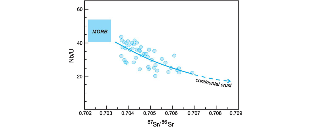
87Sr/86Sr versus Nb/U for basalts from the Society Islands (data from White and Duncan, 1996; modified after Hofmann, 2014; with permission from Elsevier). The curved trend in the basaltic data shown here is consistent with mixing between a depleted mantle component represented by MORB and a continental crustal component.
6.3.5.4 Coupled versus Decoupled Isotope Behaviour
When covariant isotopic systems that are expected to behave similarly do not, they are considered to be ‘decoupled’. Sm–Nd and Lu–Hf isotopes normally represent a coupled system, but early in Earth history they may have been decoupled with Lu–Hf isotopes showing supra-chondritic compositions, whereas Sm–Nd isotopes show chondritic compositions. Hoffmann et al. (2010, 2011) suggested that Eoarchean rocks in west Greenland were decoupled with respect to whole-rock Nd and Hf isotopes. Caro and Bourdon (2010) explained this observed decoupling of the Nd–Hf systems in terms of a supra-chondritic Earth model. However, Lu–Hf isotopes in meteoritic zircon (Iizuka et al., 2015) support the CHUR parameters of Bouvier et al. (2008) and recent Hf-in-zircon work does not reproduce supra-chondritic εHf values for the same west Greenland samples (Kemp et al., 2019); therefore, invoking a supra-chondritic Hf reservoir seems unnecessary.
6.3.6 Crust–Mantle Geodynamics
The ultimate goal of defining crust and mantle isotopic reservoirs is to create geodynamic models which explain how these reservoirs have obtained their present-day compositions and how they interact. This requires us to think about Earth processes on a global, rather than local, scale and points to a major success of isotope geology: linking reservoir compositions to the processes that govern plate tectonics. These include the subduction of oceanic crust and its associated sediment, the upwelling of mantle plumes and the recycling of continental lithosphere. We have shown in this chapter how the study of radiogenic isotopes in basalts and mantle peridotites allows us to characterize mantle end-member compositions and explore the chemical evolution of the mantle through time. These data demonstrate how the composition of the mantle has evolved in response to the processes of core formation, crust extraction and the recycling of crustal material, and it is to these themes that we now turn.
6.3.6.1 The Secular Variation of the Mantle
We showed in Section 6.3.2 that the Earth’s mantle can be characterised using the isotopes of Nd, Hf, Sr, Pb and Os into four distinct reservoirs: the depleted mantle (DM), mantle with a high 238U/204Pb ratio (HIMU) and enriched mantle reservoirs (EM1 and EM2). Each of these mantle reservoirs records its own ‘story’ of the processes which have led to its current composition, although it is important to note that to date these ‘stories’ are only partially told. The DM is thought to record events which relate to crust extraction, whereas the HIMU mantle records events of U gain or Pb loss through the in-mixing of altered oceanic crust or the loss of lead to the core or through fluid processes. There are also several models for the origin of the enriched mantle (EM) which include the recycling of crustal materials, enrichment by the migration of mantle melts and the mixing of sub-continental lithosphere into the mantle.
In Section 6.3.3 we described a range of ‘mantle evolution diagrams’ which summarise how the composition of the mantle has evolved over time for the different isotopic systems. We proposed that the Nd and Hf systems record, at least in part, the process of crust extraction and that Os isotopes can be an important tracer of recycled ancient oceanic crust. The more complex Pb isotopes record the evolution of mantle domains with different μ values over time.
Both these approaches to the composition of the modern mantle are based upon a chondritic (CHUR) model of the Earth, although, as we have indicated, studies of Hf isotopes have sought to challenge this assumption. This leads us to the starting point for all modern geodynamic models which are the large-scale processes which took place during the early differentiation of the Earth (the reader is referred to Rollinson, 2007) and whether or not any of the Earth’s primordial mantle can be recognised today.
Clues for the existence of primordial mantle come from two recent studies. A global compilation of 3He/4He, Nd and Hf isotopic data from kimberlites sampling the deeper mantle identified a homogeneous, primordial reservoir (Woodhead et al., 2019). These workers showed that this reservoir was global in extent and existed until about 200 Ma ago; it represents an ancient mantle source that remained isolated from the depleted, convecting upper mantle for about 2 Ga. It is very similar in composition to CHUR and implies that bulk Earth had a composition similar to that of enstatite chondrites (Bouvier and Boyet, 2016). McCoy-West et al. (2018) also identified a primordial mantle source in 61 Ma picrites from Baffin Island, Canada. These picrites have Sr, Nd, Hf and Pb isotopes that are indistinguishable from North Atlantic MORB, but their radiogenic W and Pb isotope compositions and their stable Fe and Zn isotope compositions are consistent with ancient primordial mantle.
6.3.6.2 The Genesis of the Continental Crust
The Sr–Nd isotope correlation diagram shown in Figure 6.10 indicates that oceanic basalts are enriched in Nd isotopes and depleted in Sr isotopes relative to the BE, whereas the rocks of the continental crust show the opposite relationship. This inverse relationship suggests that the continental crust and the mantle source of oceanic basalts are complementary reservoirs of Nd and Sr isotopes. This concept forms the basis for the mass-balance modelling of the relationship between crust, mantle and the original bulk Earth composition.
In addition to compositional constraints, the timing of crustal genesis can be addressed by the combined study of U–Pb and Hf isotopes in zircon. The key issue here is identifying juvenile crust. This can be done by using the U–Pb zircon age combined with the initial 176Hf/177Hf ratio and model age of the same zircon. Where these agree, a link can be made between igneous activity and the generation of new crust.
Figure 6.25 summarises a number of crustal growth curves for the production of juvenile crust throughout Earth history. There are two extreme scenarios which bracket the full range of models. The first scenario suggests that crustal growth over time is represented by the amount of crust existing today (Goodwin, 1996) and the second presumes that most of the Earth’s crust had been formed by about 4 Ga (Armstrong, 1981). The precise timing of the formation of the continental crust is still debated (Rollinson, 2017) and is linked to the even larger question of when precisely plate tectonics commenced on the Earth. Technological advances in mass spectrometry have driven this subject forward, and future investigations integrating microstructural, age and isotope tracer information from multiple isotope systems are likely to lead to continued advances in this field.
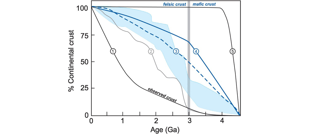
The growth of the continental crust through time. Curve 1 shows the volume of observable continental crust today (Goodwin, 1996). Curves 2–4 represent inferred crustal growth or juvenile crustal production over time (2, Condie and Aster, 2010; 3, Belousova et al., 2010; 4, Dhuime et al., 2010). Curve 5 is Armstrong’s (1981) steady-state model. The shaded region represents other crustal growth curves from Viezer and Jansen (1979), McLennan and Taylor (1982), Patchet and Arndt (1986), Chase and Patchett (1988) and McCulloch and Bennett (1994). Note the change in the rate of crust production after about 3 Ga, indicated by the vertical bar, for most models in the shaded region and models 2 and 4.
6.3.6.3 Crust and Mantle Mass-Balance Models
We have shown in this chapter the power of radiogenic isotopes in aiding our understanding of the large-scale processes operating in the Earth today. These lead to the development of geodynamic models for the Earth. Such models aim to set limits on the proportion of mantle involved in the formation of the continental crust, offer insights into the nature of mantle convection and seek to measure the rates of geological processes in order to understand how the composition of the Earth’s mantle has changed with time.
Early models such as the plumbotectonics of Doe and Zartman (1979) were based upon a single isotope system, whereas today geochemical mass-balance calculations incorporate the findings of multiple radiogenic isotope systems as well as the results of trace element and stable isotope studies. More recent studies represent exchanges between different crust and mantle reservoirs in terms of geochemical cycles and geochemical box models. Geochemical cycles are normally developed for a single element and may show cycling over a short or long time scale. Short time-scale cycles normally incorporate the reservoirs of the Earth’s surficial environment as well as the deep Earth, whereas long time-scale cycles focus on the deep Earth reservoirs. Studies of this type are augmented by geochemical box models which focus on the mass flows between the different reservoirs (see, e.g., Coltice et al., 2000). However, in order to fully understand these short- and long-term cycles we need the help of stable isotope geochemistry. This is the topic to which we now turn.