7.1 Introduction
Most naturally occurring elements consist of more than one stable isotope. In geochemistry the stable isotope systems of interest are those of the light elements H, C, N, O and S. These elements have been the subject of geochemical investigations for many decades and are termed the traditional stable isotopes. These are elements in which the mass difference between the different stable isotopes is sufficiently large to allow them to be fractionated through physical processes on the basis of their mass differences and in which the rarer isotope is of sufficient abundance to be measurable. They are often the main constituents of geologically important fluids and so provide the opportunity to study both the fluids and the effects of fluid–rock interaction.
Conventionally traditional stable isotopes are converted into a gas (usually H2, CO2 or SO2) for the purposes of isotopic analysis, and the mass differences measured in a mass spectrometer. With such commonly occurring elements as H, C, N, O and S contamination during sample preparation and analysis is a particular problem and great care must be taken to ensure clean sample handling. Increasingly, ion-beam and laser technologies are being used to obtain a finer spatial resolution of isotopic compositions in small samples. Traditional stable isotope studies typically measure the isotopic composition of a molecule or compound such as H2O or CO2 rather than the single element. This means that there are a number of different possible isotopic combinations within a single molecule. For example, carbon dioxide can exist as 12C16O2 (mass 44), as 13C16O2 or 12C17O16O (both mass 45), and there are many more possibilities. These different molecules are known as isotopologues; that is, they are molecules that differ from one another only in isotopic composition and may have the same or different masses. However, their abundances vary greatly. In the example given above, 12C16O2 makes up 98.4‰ of naturally occurring CO2, whereas 13C16O2 and 12C17O16O form only 1.11‰ and 748 ppm, respectively.
With the advent of multi-collector ICP-MS technology, a number of elements with higher atomic numbers, whose stable isotope variations had been regarded previously as too low to measure accurately, have been shown to have natural isotopic variations and added to the geochemical toolbox. These are often termed the non-traditional stable isotopes. Many occur as trace elements, some are redox sensitive, and some are biologically active, and because of their metallic nature some represent different bonding environments from the traditional covalently bonded stable isotopes. There are a large number of elements crowding into this field, with others emerging. Here we consider five of the non-traditional stable isotopes – the light elements Li, Mg and Si and the heavier elements Cr and Fe – to illustrate their diverse applications in modern geochemistry.
In this chapter we first consider in Section 7.2 some of the key principles behind interpreting stable isotope geochemistry, then in Section 7.3 there is a discussion of the application of the traditional stable isotopes H, C, N, O and S. This is followed in Section 7.4 by a discussion of the application of the non-traditional stable isotopes Li, Mg, Si, Cr and Fe. More detailed treatments of the traditional stable isotopes are given by Valley et al. (1986), Taylor et al. (1991), Sharp (2017) and Hoefs (2018), and for the non-traditional stable isotopes, Teng et al. (2017a).
7.2 Principles of Stable Isotope Geochemistry
7.2.1 Notation
7.2.1.1 Isotope Ratios: The δ Value
Stable isotope ratios are measured relative to a standard, and because the relative differences are normally very small, they are expressed in parts per thousand (informally as ‘per mil’): ‰. The isotope ratio is expressed as a δ (delta) value, or del value as it is sometimes colloquially called. Using oxygen isotopes as an example, the δ value is calculated as follows:
Thus a δ18O value of +10.0‰ means that the sample is enriched in the 18O/16O ratio relative to the standard by 10 parts in thousand and is isotopically ‘heavy’. Similarly, a negative value of −10.0‰ means that the sample is depleted in the 18O/16O ratio relative to the standard by 10 parts in a thousand and is isotopically ‘light’.
7.2.1.2 The Fractionation Factor α
The fractionation of an isotope between two substances A and B can be defined by the fractionation factor
For example, in the reaction in which 18O and 16O are exchanged between magnetite and quartz, the fractionation of 18O/16O between quartz and magnetite is expressed as
where ‘18O/16O in quartz’ and ‘18O/16O in magnetite’ are the measured isotopic ratios in coexisting quartz and magnetite. If the isotopes are randomly distributed over all the possible atomic positions in the compounds measured, then α is related to an equilibrium constant K such that
where n is the number of atoms exchanged. Normally, exchange reactions are written such that only one atom is exchanged, in which case α = K, and the equilibrium constant is equivalent to the fractionation factor.
Values for α are close to unity and typically vary in the third decimal place. Most values therefore are of the form 1.00X. For example, the fractionation factor for 18O between quartz and magnetite at 500°C is 1.009 (Javoy, 1977). This may be expressed as the third decimal place value – the per mil value – such that the quartz–magnetite fractionation factor is 9 (or 9.0 per mil). A useful mathematical approximation for the fractionation factor α stems from the following relationship:
In the case cited above where α = 1.009, 1000 ln α = 9.0. Experimental studies have shown that 1000 ln α is a smooth and often linear function of 1/T2 for mineral–mineral and mineral–fluid pairs. This gives rise to the general relationship for the fractionation factor
where T is in Kelvin and A and B are constants, normally determined by experiment. In the case of the quartz–magnetite pair the values for A and B are 6.29 and 0, respectively (Chacko et al., 2001), giving the expression:
A further useful approximation is the relationship between 1000 ln α and measured isotope ratios expressed as δ values. The difference between the δ values for two minerals is expressed as Δ which approximates to 1000 ln α, when the δ values are less than 10. In the case of oxygen isotopic exchange between quartz and magnetite,
When δ values are larger than 10, then the following expression should be used:
A range of approaches is used to obtain stable isotope fractionation factors. These include theoretical calculations based upon models of atomic structure and bond strength, experimental studies, and empirical investigations based upon well-studied natural samples (see Chacko et al., 2001, for a review; Sharp 2017). These authors also provide a helpful compilation of self-consistent, experimentally determined mineral–mineral fractionation factors (values for A) for oxygen isotopes, which is summarised here in Table 7.1.
| Cc | Ab | Ms | F-Phl | An | Phl | Ap | Zn | Alm | Di | Gr | Gh | Ttn | Fo | Ru | Mt | Pv | |
|---|---|---|---|---|---|---|---|---|---|---|---|---|---|---|---|---|---|
| Qz | 0.38 | 0.94 | 1.37 | 1.64 | 1.99 | 2.16 | 2.51 | 2.64 | 2.71 | 2.75 | 3.15 | 3.50 | 3.66 | 3.67 | 4.69 | 6.29 | 6.80 |
| Cc | 0.56 | 0.99 | 1.26 | 1.61 | 1.78 | 2.13 | 2.26 | 2.33 | 2.37 | 2.77 | 3.12 | 3.28 | 3.29 | 4.31 | 5.91 | 6.42 | |
| Ab | 0.43 | 0.70 | 1.05 | 1.22 | 1.57 | 1.70 | 1.77 | 1.81 | 2.21 | 2.56 | 2.72 | 2.73 | 3.75 | 5.35 | 5.86 | ||
| Ms | 0.27 | 0.62 | 0.79 | 1.14 | 1.27 | 1.34 | 1.38 | 1.78 | 2.13 | 2.29 | 2.30 | 3.32 | 4.92 | 5.43 | |||
| F-Phl | 0.35 | 0.52 | 0.87 | 1.00 | 1.07 | 1.11 | 1.51 | 1.86 | 2.02 | 2.03 | 3.05 | 4.65 | 5.16 | ||||
| An | 0.17 | 0.52 | 0.65 | 0.72 | 0.76 | 1.72 | 1.51 | 1.67 | 1.68 | 2.70 | 4.30 | 4.81 | |||||
| Phl | 0.35 | 0.48 | 0.55 | 0.59 | 0.99 | 1.34 | 1.50 | 1.51 | 2.53 | 4.13 | 4.64 | ||||||
| Ap | 0.13 | 0.20 | 0.24 | 0.64 | 0.99 | 1.15 | 1.16 | 2.18 | 3.78 | 4.29 | |||||||
| Zn | 0.07 | 0.11 | 0.39 | 0.86 | 1.02 | 1.03 | 2.05 | 3.65 | 4.16 | ||||||||
| Alm | 0.04 | 0.32 | 0.79 | 0.95 | 0.96 | 1.98 | 3.58 | 4.09 | |||||||||
| Di | 0.28 | 0.75 | 0.91 | 0.92 | 1.94 | 3.54 | 4.05 | ||||||||||
| Gr | 0.47 | 0.63 | 0.64 | 1.66 | 3.26 | 3.77 | |||||||||||
| Gh | 0.16 | 0.17 | 1.19 | 2.79 | 3.30 | ||||||||||||
| Ttn | 0.01 | 1.03 | 2.63 | 3.14 | |||||||||||||
| Fo | 1.02 | 2.62 | 3.13 | ||||||||||||||
| Ru | 1.60 | 2.11 | |||||||||||||||
| Mt | 0.51 |
Isotopic fractionations between minerals and melt vary as a result of the changing composition of the melt. Mineral–melt fractionations are defined in the same way as for mineral pairs (Eq. 7.2) and these values are particularly useful when seeking to calculate the stable isotope composition of a melt from the isotopic composition of one or more refractory or phenocryst phases. Other approaches used to measure the isotopic composition of a melt include the direct measurement of the fresh glass, or to treat the melt as a mixture of normative minerals with a fractionation factor calculated from the weighted average of the fractionation factors of the normative minerals (Bindeman, 2008).
7.2.2 Equilibrium Stable Isotope Fractionation
One of the most fundamental concepts behind stable isotope fractionation is that the mass of an atom affects its translational, rotational and vibrational motions and thus the strength of its chemical bonds. Most isotopic fractionations are the result of equilibrium effects and follow the rules of equilibrium thermodynamics. This means that equilibrium fractionation between two phases is based upon the differences in the bond-strength of the different isotopes of the element. The heavier isotope will form the stronger, stiffer bond. So that when an isotope is partitioned between two minerals in an exchange reaction such as
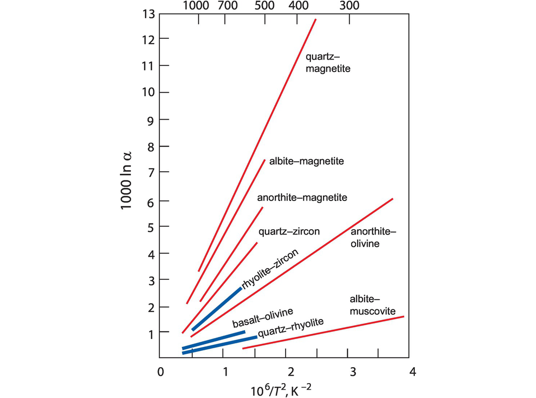
the heavier isotope will partition into the mineral with the higher ionic potential. In the case of the fractionation of 18O between quartz and magnetite, it is the quartz, which contains small highly charged Si4+, that is enriched in 18O, and the magnetite is 18O-deficient. The relationship between bond strength and isotopic fractionation was illustrated by Bindeman (2008), who gives the example of a granite at 850°C with a whole rock δ18O value of 7.8‰ which shows decreasing δ18O of its constituent minerals according to the increasing number of non-Si–O bonds in the mineral as follows:
It is evident from the above that the oxygen isotope composition of plagioclase is a function of its anorthite content.
It was shown in Eq. 7.5 that there is an important temperature control on isotopic fractionation leading to an obvious application in isotopic thermometry. Relative volume changes in isotopic exchange reactions, on the other hand, are very small, except for hydrogen isotopes, and therefore there is a minimal pressure effect. Clayton (1981) showed that at pressures of less than 20 kb the effect of pressure on oxygen isotope fractionation is less than 0.1‰ and lies within the measured analytical uncertainties. The absence of a significant pressure effect on stable isotope fractionation means that isotopic exchange reactions can be investigated at high pressures where reaction rates are fast and the results extrapolated to lower pressures.
There is also some evidence for crystallographic controls on isotope fractionation in minerals. Heavy isotopes are concentrated in more closely packed crystal structures as illustrated by the fractionation of carbon isotopes between diamond and graphite and 18O between α- and β-quartz. In calcite, crystal faces from different crystallographic forms have different isotopic compositions indicating that different surfaces in the same crystal can have slightly different bonding characteristics which are sufficient to fractionate the isotopes of oxygen and carbon (Dickson, 1991).
7.2.3 Kinetic Controls on Stable Isotope Fractionation
Kinetically controlled stable isotope fractionation reflects the readiness of a particular isotope to react and can be important in identifying particular physical and biological processes. For example, in a physical process such evaporation, an isotopically light molecule will have a slightly greater velocity than an equivalent heavy molecule. Kinetic isotope effects are often associated with fast, incomplete or unidirectional processes such as evaporation, diffusion and dissociation reactions, and unlike equilibrium processes they do not follow well-understood thermodynamic rules. Typically, they are more important in low-temperature geochemistry and are rarer at high temperatures. During distillation the light isotopic species is preferentially enriched in the vapour phase according to the Rayleigh fractionation law (Section 4.2.2) as is found in the fractionation of δ18O and δD in rainwater and ice.
When isotopic fractionation takes place as a result of diffusion, there is a kinetic effect whereby the light isotope is enriched relative to the heavy in the direction of transport indicating the mass dependence of this process (Watkins et al., 2017). At high temperatures diffusion-controlled isotopic fractionation can be important when interpreting the results of oxygen isotopes as thermometers or in experiments where high-temperature processes have not reached equilibrium. At lower temperatures isotopes can be fractionated by adsorption onto clay minerals in sediments. For example, isotopically lighter hydrogen, oxygen and sulphur may be preferentially adsorbed onto clay, leading to isotopic enrichments in formation waters (Ohmoto and Rye, 1979).
Kinetically controlled stable isotope fractionation is particularly important during biological processes and so is relevant to all the traditional stable isotope systems. Products from bacterial reactions tend to be enriched in in the light isotope because the dissociation energies are lower and bonds more easily broken. For example, the bacterial reduction of seawater sulphate to sulphide proceeds 2.2‰ faster for the light isotope 32S than for 34S. For the reactions
the rate constant k1 is greater than the rate constant k2 and the ratio k1/k2 = 1.022 (Rees, 1973). The effects of this fractionation in a closed system may be modelled using the Rayleigh fractionation equation (Section 4.2.2).
7.2.4 Mass-Independent Stable Isotope Fractionations
Some elements have more than two stable isotopes. For example, oxygen has three isotopes – 16O, 17O and 18O – and sulphur has four – 32S, 33S, 34S and 36S. Given that isotope fractionations are a function of the mass difference between the isotopes, we might expect the fractionation of 17O relative to 16O to be half that of 18O relative to 16O. Broadly, this mass-dependent fractionation is found to be the case, although with some minor differences because of the complex way in which fractionation factors relate to isotopic mass. For this reason the fractionation of 17O/16O relative to 18O/16O is 0.52, rather than precisely 0.5. However, there are some rare circumstances in which isotopic fractionation does not follow this pattern and instead represents the process of mass-independent fractionation. This has been found in the case of oxygen isotopes and sulphur isotopes where they occur in the upper atmosphere.
In geochemistry the recognition of mass-independent fractionation in the sulphur isotope system has huge importance. In this system mass-independent fractionation is quantified using the Δ-notation in the expressions
where 0.515 represents the fractionation of 33S to 34S and 1.91 represents the fractionation of 36S to 34S. These terms may be obtained by calculating the slope for pairs of measured δ3xS values in natural materials (see Farquhar and Wing, 2003, figure 2). In the modern Earth, Δ33S and Δ36S are zero, but in the early history of the Earth they have both positive and negative values (Farquhar and Wing, 2003). One helpful way of presenting the data is to plot a δ34S versus Δ33S diagram (Figure 7.24) as this shows the degree of mass-independent fractionation relative to that of mass-dependent fractionation.
Current thinking attributes the mass-independent fractionation of sulphur isotopes to photochemical reactions in the upper atmosphere (Ono, 2017); see Section 7.3.4.4. The changing pattern of mass-independent sulphur isotope evolution over time is therefore thought to relate to the chemical evolution of the Earth’s atmosphere. Experimental studies show that photolysis reactions in the ultraviolet range are capable of producing large mass-independent fractionations. This observation suggests that Earth’s ozone layer, which protects the planet from damaging ultraviolet radiation, was not present in the early Earth, supporting the view that the Earth’s early atmosphere was not oxygenic.
7.2.5 Clumped Isotopes
A relatively recent finding in stable isotope geochemistry is that there is a tendency for isotopologues containing rare heavy isotopes to concentrate more than one rare isotope in a given molecule. These ‘multiply substituted isotopologues’ have been termed ‘clumped isotopes’, the term ‘clumped’ indicating that two rare isotopes are bonded together (Eiler, 2007). The concentrations of such isotopologues are extremely low and present certain analytical challenges. In the past the assumption had been that the different isotopologues of a given molecule are randomly distributed according to their abundances in nature, whereas the recent finding is that heavy isotope isotopologues are more abundant than predicted from a purely random distribution. This can be explained by the preferential bonding of heavy isotopes in a given molecule leading to the ‘clumping’ of heavy isotopes into multiply substituted isotopologues at the expense of singly ubstituted isotopologues (Eiler, 2007).
Clumped isotope analysis uses the Δ notation to express deviation of the measured amount from that expected from the stochastic distribution. Values may be positive or negative. One of the most commonly measured values is the Δ47 value for CO2, which largely reflects variations in abundance of 13C18O16O = mass 47. The Δ47 value of CO2 can be calculated from the expression
where R47, R46 and R45 are the 47/44, 46/44, 45/44 ratios, respectively, for CO2 and R47*, R46* and R45* are the corresponding ratios if the sample had a stochastic distribution and are calculated from measured abundance ratios (see Eiler, 2007, for details). Inasmuch as clumped isotopes use the Δ notation, they might be considered similar to mass-independent isotope measurements. However, the two are very different. Clumped isotopes measure the deviation from the expected random distribution, whereas mass-independent isotope measurements record deviations from values expected from mass-dependent fractionation.
One of the main applications of clumped isotope studies is in low-temperature carbonate thermometry, giving rise to the field of ‘carbonate clumped isotope thermometry’. The formation of carbonate ions containing the heavy isotopes 13C and 18O is temperature-dependent but is independent of the fluid or mineralogical context in which the exchange reaction takes place. This allows, for example, foraminifera to be used to calculate former ocean temperatures (Meinicke et al., 2020). The novelty of this methodology means that it continues to develop both in the application of new technologies for the precise measurement of small isotopic difference and in the refinement of the equilibrium reaction to take account of impurities in the carbonate phases (Hill et al., 2020).
7.3 Traditional Stable Isotopes
7.3.1 Oxygen
The ‘vital statistics’ of oxygen isotopes, summarising the range of isotopes, the measured isotope ratio, the standards used and the range of natural compositions, are summarised in Box 7.1.
Oxygen is liberated from silicates and oxides through laser-fluorination and then reduced to CO2 at high temperature for measurement in a gas source mass spectrometer. In carbonates carbon dioxide is liberated with >103‰ phosphoric acid. When oxygen isotope ratios are determined in water, the sample is equilibrated with a small amount of CO2 and the oxygen isotope ratio in the CO2 is measured. From the known water–CO2 fractionation factor the 18O/16O ratio in the water is calculated. Isotopic measurements are carried out using gas source mass spectrometry with a precision of the order of 0.1‰ (Sharp, 2017). In situ oxygen isotope analysis is also routinely carried out by ion microprobe with a precision of 0.15–0.24‰.
In this section we consider the extent to which oxygen isotopes vary in nature, their use in high-temperature and low-temperature thermometry and their application to the understanding of magmatic processes. In particular, we consider the process of crustal contamination and how it might be demonstrated on oxygen isotope–radiogenic isotope diagrams.
7.3.1.1 Variations of δ18O in Nature
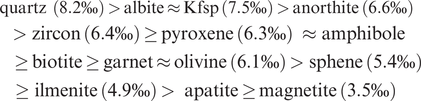
δ18O values vary in nature by about 100‰ with about half of this range occurring in meteoric water (Figure 7.1). Evidence from the analysis of ocean basalts indicates that the mantle δ18O value is 5.7 ± 0.2‰ (Bindeman, 2008), similar to the value for lunar basalts and constant over geological time (Taylor, 1980). The bulk δ18O value of chondritic meteorites is similar or slightly lighter than that of the Earth’s mantle. Felsic magmas show a broader and more positive range of δ18O values than is found in mafic and ultramafic rocks, and, similarly, sedimentary rocks and meta-sediments are isotopically heavier than mafic rocks and the mantle. Natural waters have very variable oxygen isotope compositions, as discussed below in Section 7.3.2.3, and some water types have strongly negative values relative to the VSMOW standard.
Stable isotopes and abundances
Measured isotope ratio
Standard
Vienna Standard Mean Ocean Water (VSMOW), which has an absolute 18O/16O ratio of 0.020052 (Baertschi 1976)
PDB: a belemnite from the Cretaceous Peedee formation of South Carolina (used for low-temperature carbonates)
Mantle value
Variations in nature
See Figure 7.1.
The distribution of oxygen isotopes in the major terrestrial reservoirs relative to the Earth mantle (δ18O‰ =5.7 ± 0.2 VSMOW).
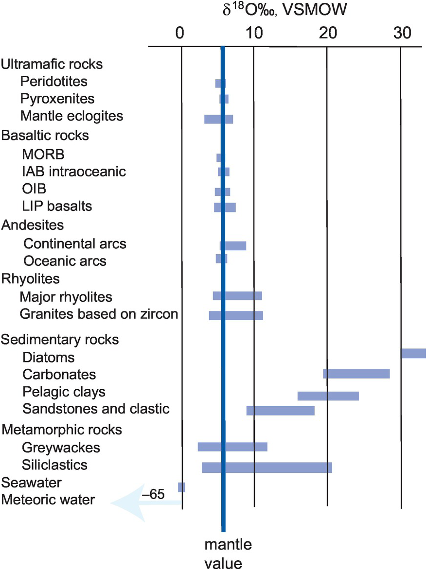
From these observations we can infer that crustal rocks with high δ18O values (i.e., those that are isotopically heavy) must have experienced some interaction with or were in part derived from high-δ18O metasedimentary silicate rocks such as meta-pelites or greywackes. Equally, there are a smaller number of crustal rocks which have unusually low δ18O values, that is, below mantle values. These are thought to represent samples which have interacted with a low-δ18O reservoir, the main contender for which is meteoric water. This interaction could be through the hydrothermal alteration of the parent rocks or the metamorphism and/or re-melting of hydrothermally altered source materials (Ryan-Davis et al., 2019). In both instances it is evident that rocks which deviate significantly away from mantle values must have experienced some interaction with materials at the Earth surface, illustrating the way in which oxygen isotopes can be a useful monitor of the process of crustal assimilation and contamination. This was demonstrated by Bindeman (2008), who showed that the assimilation of high-δ18O supracrustal materials and low-δ18O hydrothermally altered rocks gives rise to high- and low-δ18O magmas, respectively (Figure 7.2).
A δ18O versus SiO2 plot showing the field of mid-ocean ridge basalts (MORB) and the normal array of intermediate to felsic magmas. Also shown are the manner in which high-δ18O melts are produced by the assimilation of high-δ18O supracrustal materials and low-δ18O melts are the product of the assimilation of low-δ18O hydrothermally altered rocks.
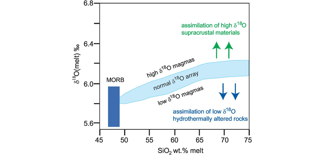
A particularly important means of recovering the δ18O value of a magma is through the measured oxygen isotope composition of the minerals zircon and quartz. This is possible because (i) these minerals preserve their δ18O even through high grades of metamorphism (Valley, 2003) and (ii) at high temperatures the fractionation of δ18O between zircon or quartz and melt is small (Figure 7.3). An empirical study by Bindeman and Valley (2002) suggests that the δ18O of a rhyolitic melt is about 2‰ higher than that of the zircon at ~750°C and slightly less at higher temperatures. Similarly, the δ18O of quartz almost mirrors that of the melt, in particular, at temperatures >850°C (Bindeman, 2008). This approach is particularly important in the study of detrital zircons where their magmatic provenance is unknown (Valley, 2003).
Fractionation factors expressed as 1000 ln α plotted relative to temperature shown as °C on the top axis and as 106/T2 Kelvin on the lower axis. Mineral–mineral fractionation factors are shown as red lines and mineral–melt fractionation factors as blue lines.
7.3.1.2 Oxygen Isotope Thermometry.
One of the first applications of the study of oxygen isotopes to geological problems was to geothermometry. In 1947 Urey suggested that the enrichment of 18O in calcium carbonate relative to seawater was temperature-dependent and could be used to determine the temperature of ancient ocean waters. The idea was quickly adopted, and palaeo-temperatures were calculated for the Upper Cretaceous seas of the Northern Hemisphere. Subsequently, a methodology was developed for application to higher-temperature systems based upon the distribution of 18O between coexisting mineral pairs. An excellent review of the methods and applications of oxygen isotope thermometry is given by Clayton (1981).
The expression summarising the temperature dependence of oxygen isotope exchange between a mineral pair was given above as Eq. 7.5 and is summarised in the expression
where T is in Kelvin and A and B are constants. Often the ‘B’ term is zero, making the fractionation factor simply a function of 1/T2.
Empirical observations indicate that a graph of ln α versus 1/T2 is linear over a temperature range of several hundred degrees (Figure 7.3) and a plot of this type for a pair of anhydrous phases should pass through the origin. Isotopic fractionations decrease with increasing temperature, and so oxygen isotope thermometers might be expected to be less sensitive at high temperatures. However, experimental studies are most precise at high temperatures (see, e.g., Clayton et al., 1989), and so thermometers have been calibrated for use with igneous and metamorphic rocks. Temperature estimates are most reliable for mineral pairs with large 1000 ln α values, such as the mineral pair quartz–magnetite (Figure 7.3).
(a) High-temperature applications of oxygen isotope thermometry. Initially, it was thought that oxygen isotope thermometry in igneous and metamorphic rocks had a number of advantages over conventional cation-exchange thermometry since there was the potential for oxygen isotopic exchange to be measured between many different mineral pairs in a single rock. However, subsequent studies have shown that the re-equilibration of oxygen isotopes between mineral pairs during cooling means that peak conditions in metamorphic rocks and magmatic temperatures in igneous rocks are not always recorded. This means that for oxygen isotope thermometry to reliably record high-temperature events, the minerals examined must be primary and unaltered; they must have not experienced exchange with a fluid phase; and the rock or magma cooled quickly so the measured isotope values are quenched and do not represent later diffusion. These conditions are rarely met for metamorphic and plutonic rocks, although they can be applied to fresh volcanic rocks containing quenched phenocrysts.
Several tests have been proposed for the reliability of oxygen isotope thermometry, the most useful of which is the concordance test and is based on the observation that there are potentially a large number of thermometers available in a single rock. The method uses mineral-pair measurements plotted on an isotherm plot in order to examine concordance between the different mineral-pair measurements and to assess the extent of isotopic equilibrium (Javoy et al., 1970; Huebner et al., 1986; Gregory et al., 1989). Isotopic equilibrium is measured relative to a straight line with a slope = 1.0, and any departure from this trend is indicative of isotopic disequilibrium.
Currently, the main application of high-temperature oxygen isotope thermometry is focused on refractory mineral pairs in which oxygen diffusion rates are low and which have seen no interaction with fluids. The selection of suitable mineral pairs therefore must be made on the basis of the expected temperature range to be determined in the light of diffusion rates and mineral closure temperatures (Valley, 2001). Suitable minerals include aluminosilicates, magnetite, garnet and rutile in quartzite, and magnetite, titanite and diopside in marble. In igneous rocks the minerals quartz and zircon may be used in silicic rocks and olivine in mafic rocks (Valley, 2001). A plot of measured and empirical mineral–mineral and mineral–melt fractionations versus temperature is shown in Figure 7.3, and a table of relevant fractionation factors is given in Table 7.1 (after Chacko et al., 2001, and Valley, 2003). A recent addition to these fractionation factors is the work of Lacroix and Vennemann (2015), who made an empirical estimate of the fractionation between quartz and Fe–Mg chlorites. They show that for the temperature range 240–550°C,
A coexisting quartz–orthopyroxene pair from a granulite facies metapelite (Huebner et al., 1986, sample Bb25c) has the following measured compositions:
The temperature dependence on the fractionation of 18O between quartz and pyroxene (we use the diopside value as an approximation) – see Table 7.1 and Eq. 7.5 – is
Since the δ value for quartz is >10.0, in this case we use Eq. 7.7
thus
and
From the thermometer equation (7.5)
(b) Low-temperature applications of oxygen isotope thermometry. The earliest application of oxygen isotopes to geological thermometry was in the determination of ocean palaeotemperatures. The method assumes isotopic equilibrium between the carbonate shells of marine organisms and ocean water and uses the equation of Epstein et al. (1953). This equation is still applicable despite some proposed revisions (Friedman and O’Neill, 1977):
where δc and δw are respectively the δ18O of CO2 obtained from CaCO3 by reaction with H3PO4 at 25°C and the δ18O of CO2 in equilibrium with the seawater at 25°C. The method assumes that the oxygen isotopic composition of seawater was the same in the past as today, an assumption which has frequently been challenged and which does not hold for parts of the Pleistocene when glaciation removed 18O-depleted water from the oceans (Clayton, 1981). The method also assumes that the isotopic composition of oxygen in the organism is the same as in seawater and ignores any species specific ‘vital effects’, and that there has not been any post-burial isotopic exchange with sediment pore water. Because the temperatures of ocean bottom waters vary as a function of depth, it is also possible to use oxygen isotope thermometry in palaeobathymetry to estimate the depth at which certain benthic marine fauna lived.
Using these methods, the careful analysis of deep sea sediment cores has allowed us to reconstruct past ocean temperatures and thus past climates over at least 800,000 years and shows the cyclicity of glacial and interglacial periods. Similarly, climatologists have recognised that continental glacial ice also preserves a long-term record of climate change, which shows the same cyclicity as seen in marine cores. In these studies both δ18O and δD (see Section 7.3.2) are used as temperature proxies. δ18O ice-core measurements are converted into temperature using a calibration based upon the linear relationship between annual values for δ18O and mean annual temperature at the precipitation site (Jouzel et al., 1997) in which δ18O becomes more negative with decreasing temperature. One such linear relationship for the Greenland Summit area gives the relationship δ18O‰ = −148.04 + 0.46403T (K). While this modern analogue method works best at middle to high latitudes, there are other local (geographic) and temporal factors that must be taken into account in order to obtain an accurate temperature estimate in other areas (Jouzel et al., 1997).
7.3.1.3 Oxygen Isotope–Radiogenic Isotope Correlation Diagrams
Correlations between radiogenic and oxygen isotopes are of particular importance because variations in the two types of isotope come about through totally different mechanisms and they are particularly important in recognising processes that involve contamination and mixing.
(a) Recognising crust and mantle reservoirs. Oxygen isotopes are a very effective way of distinguishing between rocks which formed in equilibrium with the mantle and those which formed from the continental crust. In general, the continental crust is enriched in δ18O relative to the Earth’s mantle (Figure 7.1). This has come about largely as a consequence of the long interaction between the continental crust and the hydrosphere and the partitioning of 18O into crustal minerals during low-temperature geological processes. Oxygen isotopes, therefore, are a valuable indicator of surface processes and a useful tracer of rocks which at some time have had contact with the Earth’s surface. Radiogenic isotopes, on the other hand, show differences between crust and mantle reservoirs which are a function of long-lived differences in parent–daughter element ratios and indicate the isolation of the reservoirs from one another for long periods of Earth history. This gives rise to crustal reservoirs which generally are enriched in 87Sr/86Sr and in radiogenic lead isotopes but depleted in 143Nd/144Nd and 176Hf/177Hf relative to the mantle. As an example, the range of combined oxygen and strontium isotopic compositions in common rock types is shown in Figure 7.4.
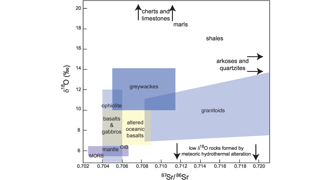
The indicative ranges of oxygen and strontium isotopes in common igneous and sedimentary rocks.
(b) Recognising crustal contamination in igneous rocks. Many crustal materials have oxygen and strontium isotope ratios which differ from mantle values (Figure 7.4) and so have the potential to provide evidence of the interaction between mantle rocks and the continental crust. This interaction may be through the contamination of mantle-derived melts in the continental crust or through the contamination of the source region by the subduction of crustal materials into the mantle. Details of the mixing processes are given by Taylor (1980), James (1981) and Taylor and Sheppard (1986).
The calculation of mixing curves entails some assumptions about the relative proportions of the parent element of the radiogenic isotope in the end-member compositions. In the case of strontium, when the contaminant in a source region is enriched in Sr relative to the mantle and forms a relatively small proportion of the whole, then contamination on a 87Sr/86Sr versus δ18O mixing diagram is characterised by the convex downward curvature of the mixing line. This arises because not only are crustal materials enriched in Sr relative to the mantle but their 87Sr/86Sr ratio is greater than that of the mantle and thus dominates any mixture of the two. Oxygen concentrations, however, are broadly similar in all rocks so that there is no large increase in the oxygen isotope ratio of the derivative melt. The small increase in δ18O is a simple linear function of the bulk proportion of crustal to mantle materials. In the case when the melt is enriched in Sr relative to the contaminant and the relative proportion of the contaminant is high, then compositions on a Sr–O isotope plot will define a mixing curve with a convex-up curvature (James 1981). This could be the case for a mantle-derived melt passing through the continental crust.
An example of the way in which source mixing has been inferred using oxygen and radiogenic isotopes is given by Trumbull et al. (2004). They show that 130 Ma, Cretaceous granites and related rhyolitic lavas from Namibia have a range of compositions that implies the mixing of mafic melts similar to those found in the Tristan mantle plume with a melt of lower crustal felsic rocks similar in composition to the A-type Damaran granites found in this region. A plot of δ18O in quartz versus the whole-rock Nd isotope composition, expressed as εNd, for a range of granitoids and felsic lavas lies on a mixing line between the probable mantle source and a lower crustal source (Figure 7.5a). A similar trend is seen on a plot of δ18O versus the Sr isotope composition of the melt at 130 Ma (Figure 7.5b) and illustrates the convex-downward mixing curve described above.
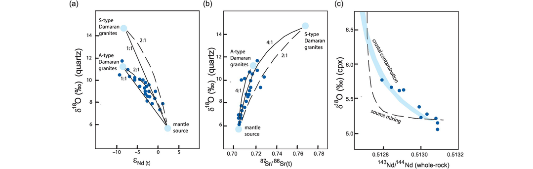
δ18O versus radiogenic isotopes. (a) Plot of δ18Oquartz versus εNd(t) for granitoids and felsic volcanic rocks (dark blue symbols) from Namibia. Source compositions for the mantle and two proxy crustal sources (Damaran granites) are shown in pale blue. Mixing lines between the mantle and crustal sources are constructed for the cases when the Nd concentrations in the crust and mantle are the same (1:1) and when the Nd concentration in the mantle is twice that in the crust (2:1). (b) Plot of δ18Oquartz versus (87Sr/86Sr)130Ma for granitoids and felsic volcanic rocks (blue symbols) from Namibia. Source compositions for the mantle and two proxy crustal sources are shown in pale blue. Mixing lines between the mantle and crustal sources are constructed for the cases when the Nd concentrations in the mantle are twice (2:1) and four times (4:1) that in the crust. The data in panels (a) and (b) do not support mixing between the mantle source and melts of a lower crystal source similar in composition to the S-type Damaran granites (after Trumbull et al., 2004; with permission from Elsevier). (c) Plot of δ18Oclinopyroxene versus (143Nd/144Nd)whole-rock) for arc-related lavas from the Kermadec–Hikurangi margin (after MacPherson et al., 1998; with permission from Elsevier). Arc lavas are shown as blue symbols; the pale blue curve is the calculated trend for models of the magma contaminated by continental crust. The dashed line is the calculated curve for mixing between depleted upper mantle and fluids derived from subducted oceanic crust. The data support the crust-contamination model.
MacPherson et al. (1998) sought to discriminate between mixing in the source region and crustal contamination in the Kermadec–Hikurangi convergent margin. Using δ18O in clinopyroxene as a proxy for the composition of melts, they showed that there is a linear trend between δ18O and whole-rock 143Nd/144Nd (in modern lavas this is the same as the mantle ratio). The results were compared with mixing curves for the contamination of the source region – the mixing of a depleted mantle peridotite with a fluid derived from altered subducted oceanic crust and sediment – and the contamination of basalt with crustal sediments. They showed that the shape of the curve defined by the data gave a better fit to the curves for crustal contamination than that calculated for mixing in the source (Figure 7.5c), indicating that the melts had interacted with sediments prior to eruption.
Source contamination is more easily recognisable in regions where there is no continental crust such as in oceanic basalts. This, however, has become possible only with improved resolution in oxygen isotope analysis, for the oxygen isotope variations may be small. Studies by Eiler (2001) showed that a small increase in δ18O (less than 1.0‰) in olivine in ocean island basalts correlated with increasing 87Sr/86Sr, implies a contaminated source.
Finally, it is important to note that crustal contamination is rarely a simple mixing process and frequently involves three components: a melt, a precipitating cumulate phase and a contaminant (Taylor, 1980; James, 1981). This is the AFC process illustrated in Figure 7.6 for mixing between δ18O and 87Sr/86Sr from Taylor (1980). AFC processes, as opposed to simple mixing curves, are represented by a sigmoidal curve which does not extrapolate back to the position of either the source or contaminant.
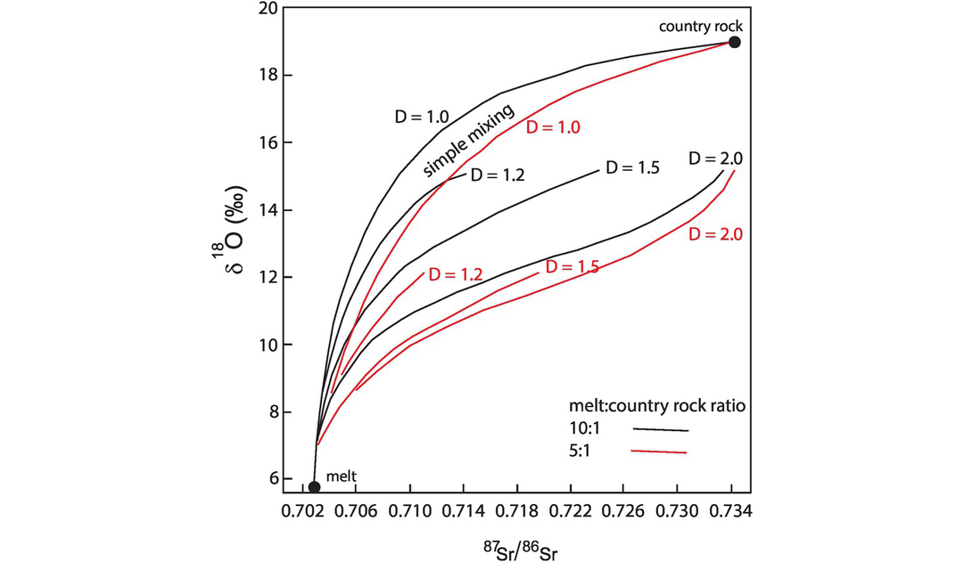
Variation in δ18O with 87Sr/86Sr during assimilation and fractional crystallisation of a magma with δ18O = 5.7 and 87Sr/86Sr = 0.703 contaminated with a crustal component (country rock) with δ18O = 19 and 87Sr/86Sr = 0.735, for values of the partition coefficient (D) for Sr from 1 to 2. The black curves are for R = 0.1 (melt to country rock ratio = 10:1) and the red curves are for R = 0.2 (melt to country rock ratio = 5:1). The ratio of cumulates to assimilated country rock is 5:1.
(c) Recognising simple crystal fractionation in igneous rocks. An igneous system which has not suffered crustal contamination will exhibit the radiogenic isotope characteristics of the source, for radiogenic isotope ratios are not altered by crystal–liquid equilibria such as crystal fractionation. Oxygen isotopes, on the other hand, do show small changes in isotope ratio with crystal fractionation as is illustrated in Figure 7.2 and show a small increase in δ18O with increasing silica content. This decoupling between oxygen and strontium isotopes was documented by Chivas et al. (1982) in a study of a highly fractionated oceanic-arc plutonic suite in which oxygen isotope ratios increase from mantle values (δ18O = 5.4‰) in gabbros to δ18O = 7.2‰ in an aplite dyke, whereas 87Sr/86Sr ratios remain constant within the limits of error of their determination.
7.3.2 Hydrogen Isotopes and the Stable Isotope Geochemistry of Water and Hydrothermal Fluids
The element hydrogen is ubiquitous in nature in the forms H2O, OH−, H2 and as hydrocarbons. There are two isotopes of hydrogen: 1H and 2H, normally referred to as D (deuterium); isotope ratios are measured as the ratio D/1H, expressed as δD. Hydrogen isotopes show the largest relative mass difference between two stable isotopes with the result that there are large variations in measured hydrogen isotope ratios in naturally occurring materials.
The study of oxygen isotopes in conjunction with the isotopic study of hydrogen has proved to be a very powerful tool in investigating geological processes involving water. When plotted on a bivariate δD versus δ18O graph, waters from different geological environments are found to have very different isotopic signatures (Section 7.3.2.3). Hydrogen is a minor component of most rocks, and so, excepting when the fluid–rock ratio is very low, the hydrogen isotope composition of rocks and minerals is sensitive to the hydrogen isotope composition of interacting fluids. Oxygen, on the other hand, comprises 50‰ by weight (and in some cases more than 90‰ by volume) of common rocks and minerals and so is less sensitive to the oxygen isotope ratio of interacting fluids, except at very high fluid–rock ratios (Section 7.3.2.6).
7.3.2.1 Hydrogen Isotopes
The basic data for hydrogen isotopes are given in Box 7.3, and a summary of δD values for solar system bodies (Figure 7.7) and common rock types and waters (Figure 7.8) are also provided. Hydrogen is generated by heating minerals in a radio frequency (RF) induction furnace to liberate water from the mineral host. The water is then reduced to hydrogen in a furnace using zinc (Vennemann and O’Neill, 1993) or uranium.
Stable isotopes and abundances
Measured isotope ratio
In hydrology δD may be referred to as δ2H
In planetary studies δD may be expressed as D/H (the conversion factor uses the absolute value for D/H recorded below and Eq. 7.14)
Standard
Mantle value
δD‰ = −76 to −48‰ (average of 61‰); recommended value −60 ± 5‰ (Clog et al., 2013).
Bulk Earth δD‰ = −43
Variations in δD in the solar system
See Figure 7.7.
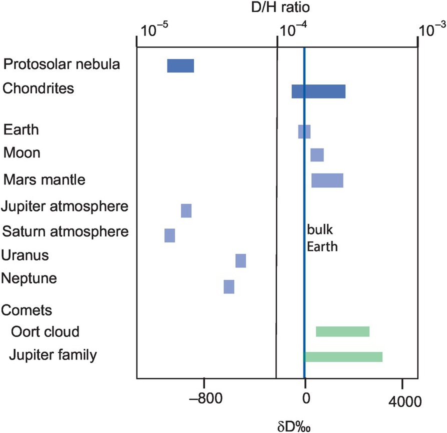
The range of hydrogen isotopes in solar system objects relative to the bulk Earth. (Data sources discussed in the text)
Terrestrial variation of δD.
See Figure 7.8
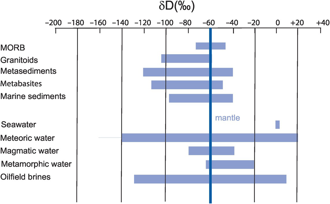
The range of hydrogen isotopes in some terrestrial reservoirs relative to the Earth’s mantle. (Data sources discussed in the text)
7.3.2.2 The Distribution of Hydrogen Isotopes in the Solar System
As might be expected, given the fundamental nature of hydrogen in the solar system, the fractionation of D/H between solar system objects is of considerable interest in planetary geochemistry, in particular, in the quest to understand the origin of water on the Earth and in other planetary bodies. There are now data from a number of solar system objects obtained by direct measurement from spacecraft and from spectral studies which show that the fractionations are very large with δD from < −800 to > +4000 and D/H varying over two orders of magnitude (Saal et al., 2013; Clarke et al., 2019). In planetary geochemistry D/H ratios are thought to indicate where in the solar system planets and different solar system objects formed. The protosolar nebula was isotopically light with D/H about 0.25 × 10⁻⁴, similar to the values recorded from the atmospheres of Jupiter and Saturn. Values for the inner solar system, including Earth and Mars, are higher but define a narrow range of D/H ratios of ~1.5 × 10⁻⁴. The D/H of the bulk Earth is 1.49(± 0.03) × 10−4 (δD = −43) (Lécuyer et al., 1998), slightly lower than the Earth’s oceans (D/H = 1.56 × 10⁻⁴). Outer solar system comets have higher values ranging from Earth-like values to D/H ~5.0 × 10⁻⁴. Carbonaceous chondrite meteorites have δD values in the range −197 to +133‰, although CI chondrites have a narrower range of between +77 and +133 (Eiler and Kitchen, 2004). These values are shown in Figure 7.7, using data from Eiler and Kitchen (2004), Usui et al. (2012), Saal et al. (2013), Altwegg et al. (2015) and Clarke et al. (2019).
7.3.2.3 The Distribution of Hydrogen Isotopes in Natural Waters
The isotopic composition of natural waters may be obtained either by direct measurement or by calculation from hydrous mineral phases using the method outlined in Section 7.3.2.5. Much of the work in this field was carried out in the 1960s and 1970s by Hugh Taylor’s group working at Caltech and is summarised in major contributions (Taylor, 1974; 1978). Taylor (1974) identifies six types of naturally occurring water which have a major influence on our thinking about hydrogeological processes, the compositions of which are summarised on a δD versus δ18O diagram (Figure 7.9). The isotopic character of the different types of water described here can be used to trace the origin of hydrothermal solutions.
(a) Ocean water. Standard Mean Ocean Water is the isotopic standard for both δ18O and δD; therefore, convention dictates that ocean water has δ18O = 0‰ and δD = 0‰. Exceptions to this rule are from areas such as the Red Sea which has elevated values of δ18O and δD created through high rates of evaporation, or from areas where seawater is diluted with fresh water. Muehlenbachs and Clayton (1976) suggested that the oxygen isotopic composition of ocean water is buffered by exchange with the ocean crust, a view which is strongly supported by the study of Gregory and Taylor (1981) on the distribution of oxygen isotopes in the Semail ophiolite, Oman (Figure 7.12).
Less certain is the isotopic composition of seawater in the past. Lécuyer et al. (1998) and Pope et al. (2012) calculated that in the very early Earth the mass of the oceans was greater by about 20‰, that the hydrogen isotope composition of seawater was lower than the present value by 20–30‰ but that the oxygen isotope composition was comparable to that of the modern oceans. In geologically more recent times there is evidence from the oxygen isotope composition of benthic foraminifera that there were global changes in the isotopic chemistry of the oceans during the Tertiary. In addition, data from marine sediment cores show that there were also changes to the oxygen isotope composition of the oceans during the Holocene brought about by the storage of isotopically light oxygen in ice in the polar regions, giving rise to isotopically heavier ocean water.
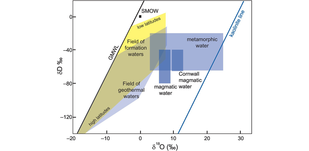
Plot of δD versus δ18O diagram for different water types. The fields of magmatic water, formation waters and geothermal waters are taken from Taylor (1974). The field for magmatic water from the granites of Cornwall is from Sheppard (1977). The metamorphic water field combines the values of Taylor (1974) and Sheppard (1981). The meteoric water line is from Craig (1961) and the kaolinite line from Taylor (1974).
(b) Meteoric water. Meteoric water shows the greatest variation in δD of all natural waters and the relationship between δD and δ18O is linear and quantified by Craig (1961) as:
δD and δ18O values for meteoric water vary according to latitude. Values are close to zero on tropical ocean islands, whereas at high latitudes in continental areas δ18O values are as low as −55‰ and δD values extend down to −440‰, although δD values below −160‰ are for polar snow and ice. Both the extreme variation and the linear relationship arise from the condensation of H2O from the Earth’s atmosphere. The extreme variation reflects the progressive lowering of 18O in an air mass as it leaves the ocean and moves over a continent. The linearity of the relationship, now known as the Global Meteoric Water Line (GMWL, Figure 7.9), indicates that fractionation is an equilibrium process and that the fractionation of D/H is proportional to 18O/16O. Subsequent studies identified deviations away from the GMWL, and some local meteoric water lines have slopes significantly different from the value of 8 due to local differences in temperature and humidity and kinetic effects during evaporation (Jouzel and Koster, 1996).
(c) Geothermal water. Modern geothermal water is meteoric in origin but isotopic compositions are transposed to higher δ18O values through isotopic exchange with the country rocks. δD values are the same as in the parent meteoric water or slightly enriched due to the non-equilibrium evaporation of water vapour (Figure 7.9). In contrast, ocean-floor geothermal systems are far more complex, particularly if methane is present, for they may host microbial communities which fractionate D/H to produce extremely light hydrogen with δD values < −400‰ (Konn et al., 2015).
(d) Formation water. Formation waters from sedimentary basins are usually saline and show a wide range in δ18O and δD values (Figure 7.9). The formation waters reported by Taylor (1974) are brines from oilfields. His results show that individual basins have water compositions which define specific linear trends representing mixing between meteoric water and either water from another source such as trapped seawater or the country rock. There is a decrease in the δD of formation waters at higher latitudes, further emphasising the link with surface meteoric waters.
(e) Magmatic water. The composition of magmatic waters is calculated from the isotopic compositions of igneous minerals (see Section 7.3.2.5). Particularly useful is the mineral muscovite, for at 800°C the isotopic composition of muscovite is the same as that of the water with which it is in equilibrium. The compositional range of magmatic water is quite well constrained for most igneous minerals and defines a very restricted field in δD–δ18O space, between −40 and −80‰ and +5.5 and +9.0‰, respectively (Taylor, 1974). Sheppard (1977), however, showed that the magmatic waters associated with the Permian granites in Cornwall, southwest England, plot in a different field with δD values of −40 to −65‰, and δ18O values of +9.5 to +13‰ (Figure 7.9). These granites are most probably the product of intra-crustal melting, and so the higher δ18O is inherited from a crustal protolith. This example highlights one of the ongoing difficulties in interpreting δD–δ18O data – that of differentiating between rocks whose source interacted with meteoric water prior to melting, that is, low-δ18O magmas, and those which interacted with meteoric water during or after emplacement. New advances in our understanding in this area have come from a study of δ18O in zircons; see, for example, Gilliam and Valley (1998) and Rumble et al. (2002).
(f) Metamorphic water. Our only access to the composition of metamorphic water is by back-calculating from the minerals present in the rock. In order to do this accurately, the temperature of the metamorphism must be known. Estimates of the δD and δ18O values of water in equilibrium with metamorphic minerals over a range of metamorphic grades have been made by Taylor (1974), Rye et al. (1976) and Sheppard (1981). A combination of these values gives a metamorphic water ‘box’ with δ18O values between +3 and +25‰ and with δD values between −20 and −65‰ (Figure 7.9). The relatively high δ18O values in some metamorphic rocks may suggest some inheritance from their sedimentary protoliths.
7.3.2.4 The Distribution of Hydrogen Isotopes in Terrestrial Reservoirs
The distribution of hydrogen isotopes from the upper mantle, the crust and clays associated with weathering is summarised in Figure 7.8 and in the discussion below.
(a) The depleted upper mantle. The δD value for the upper depleted mantle has been estimated from studies of magmatic water liberated from MORB. Early studies suggested a wide range of values but with the majority falling between −85 and −65‰ (Kyser and O’Neill, 1984). More recent measurements for the depleted upper mantle have revised these estimates and suggest a range between −76 and −48‰ with an average of 61‰ and a recommended value of −60 ± 5‰ (Clog et al., 2013). This value is close to that calculated by Lécuyer et al. (1998) for the bulk Earth of −40‰.
(b) Crustal lithologies. Other terrestrial reservoirs show a wide range of δD values, since frequently the whole-rock δD value of many terrestrial rocks is a composite value resulting from many different processes. In the case of igneous rocks, for example, processes such as magmatic degassing, crystal fractionation from a melt and sub-solidus interaction with meteoric water might all be superimposed on and thereby obscure the primary magmatic value. For this reason, the range of values for crustal lithologies shown in Figure 7.8 is not particularly useful as a discriminant.
Granitoids from the New England batholith, Australia, have δD values between −60 and −130 (O’Neill et al., 1997) and A-type granites from eastern China have δD = −59 to −145 (Wei et al., 2000). Meta-sediments have bulk rock δD values between −70 and −120 (Taylor, 1974), although lower values are recorded by Harris et al. (1997). Ultra-high-pressure (UHP) mafic rocks and felsic gneisses from the Dabie–Sulu orogenic belt in China have δD values in the range −74 to −100 (Chen et al., 2011). Lower-grade mafic and ultramafic rocks have a similar range of values (−51 to −115; Ikin and Harmon, 1983). In marine sediment δD values are in the range δD = −40 to −95 (Taylor 1974).
(c) Clay minerals in the weathering environment. There is strong relationship between the isotopic composition of kaolin in weathering zones and the coexisting meteoric waters such that it is possible to define a ‘kaolinite line’ sub-parallel to the GMWL in which, relative to meteoric waters, clays are enriched in δ18O and depleted in δD (Figure 7.9). The kaolinite line may be expressed as
The linear relationship suggests that the kaolin was formed in equilibrium with meteoric water (Taylor, 1974). In a similar way, the clay mineral smectite also forms a linear array on δ18O–δD diagrams, defining a ‘smectite line’. However, in this case the position of the smectite line is temperature-sensitive such that the distance between the GMWL and the smectite line increases with decreasing equilibration temperature and shifts towards higher δ18O values. The link between meteoric water and clay minerals means that the minerals kaolinite and smectite offer the potential to be palaeoclimatic indicators and allow for the calculation of the δ18O and δD of the meteoric water in which they were in equilibrium (Mix and Chamberlain, 2014). The temperature of kaolination can be calculated from the equation of Clauer et al. (2015):
7.3.2.5 Calculating the Isotopic Composition of Hydrothermal Fluids from Mineral Compositions
Most commonly, the δD and δ18O composition of a hydrothermal fluid has to be calculated from the isotopic composition of minerals which were in equilibrium with it using laboratory calibrations of equilibria between rock-forming minerals and water. More rarely, the isotopic composition of hydrothermal fluids can be measured directly as the fluid preserved in fluid inclusions (Ohmoto and Rye, 1974; de Graaf et al., 2019). Where isotopic compositions are calculated, it is necessary to show that there was a close approach to isotopic equilibrium between a given mineral and the original hydrothermal fluid. This is not always straightforward, for the diffusion rates of hydrogen isotopes may be up to 100 times faster than those for oxygen isotopes even in the same mineral (Kyser and Kerrich, 1991).
Experimental calibrations for both oxygen and hydrogen isotopes in a range of mineral phases are given in Tables 7.2 and 7.3, respectively, allowing the isotopic composition of a hydrothermal fluid to be fully specified. This calculation requires knowledge of the temperature of equilibration which may have to be estimated or measured independently from a technique such as fluid inclusion thermometry. An example of this approach is given by Hall et al. (1974, table 4) in a study of the origin of the hydrothermal fluids involved in the formation of the Climax molybdenum deposit, Colorado. In this study the temperature of the hydrothermal fluid was already known from fluid inclusion thermometry and the δ18O and δD composition of the water were calculated from the isotopic composition of muscovite and sericite using the experimental calibrations for muscovite–water. An example of the calculation is given in Box 7.4.
Data
δ18Omuscovite = +7.4‰
δDmuscovite = −91.0‰
Temperature = 500°C (from fluid inclusion thermometry)
Calculation of the oxygen isotope composition of the water
The equation for muscovite–water (O’Neill and Taylor, 1967; see Table 7.2) is
at 500°C
Since Δmuscovite-water = 1000 ln α
Calculation of the hydrogen isotope composition of the water
The equation for muscovite–water (Suzuoki and Epstein, 1976; see Table 7.3) is
at 500°C
Since Δmuscovite-water = 1000 ln α
| Mineral | T (°C)b | A | B | Reference | ||
|---|---|---|---|---|---|---|
| Barite | 100–350 | −6.79 | 3.00 | Friedman and O’Neill (1977) | ||
| Calcite | 0–700 | −3.39 | 2.78 | O’Neill et al. (1969) | ||
| Dolomite | 252–295 | −3.24 | 3.06 | Matthews and Katz (1977) | ||
| Quartz | 200–500 | −3.4 | 3.38 | Clayton et al. (1972) | ||
| 500–750 | −1.96 | 2.51 | Clayton et al. (1972) | |||
| 250–500 | −3.31 | 3.34 | Matsuhisa et al. (1979) | |||
| 500–800 | −1.14 | 2.05 | Matsuhisa et al.,(1979) | |||
| Alkali feldspar | 350–800 | −3.41 | 2.91 | O'Neil and Taylor (1967) | ||
| 500–800 | −3.7 | 3.13 | Bottinga and Javoy (1973) | |||
| Albite | 400–500 | −2.51 | 2.39 | Matsuhisa et al. (1979) | ||
| 500–800 | −1.16 | 1.59 | Matsuhisa et al. (1979) | |||
| Anorthite | 350–800 | −3.82 | 2.15 | O'Neil and Taylor (1967) | ||
| 400–500 | −2.81 | 1.49 | Matsuhisa et al. (1979) | |||
| 500–800 | −2.01 | 1.04 | Matsuhisa et al. (1979) | |||
| Plagioclase | 350–800 | −3.4 − 0.14 × An | 2.91 − 0.76 × An | O’Neill and Taylor (1967) | ||
| 500–800 | −3.7 | 3.13 − 1.04 × An | Bottinga and Javoy (1973) | |||
| Muscovite | 400–650 | −3.89 | 2.38 | O’Neill and Taylor (1967) | ||
| 500–800 | −3.1 | 1.9 | Bottinga and Javoy (1973) | |||
| Rutile | 575–775 | 1.46 | 4.1 | Addy and Garlick (1974) | ||
| Magnetite | 500–800 | −3.7 | −1.47 | Bottinga and Javoy (1973) | ||
| Kaolinite | 0–350 | −4.05 | 2.76 | Sheppard and Gilg (1996) | ||
| Smectite | 0–350 | −6.75 | 2.55 | Sheppard and Gilg (1996) | ||
| Illite | 0–350 | −3.76 | 2.39 | Sheppard and Gilg (1996) | ||
| Chlorite | 66–175 | For [Mg2.5Fe0.5(OH)6][Al1.5Fe1.5][Al, Si3O10][OH2] | ||||
| −11.97 + 2.67x + 2.93x2 − 0.415x3 + 0.037x4 ; where x = 103/T | Savin and Lee (1988) | |||||
| Mineral | T (°C) | A | B | Reference |
|---|---|---|---|---|
| Muscovite | 450–800 | 19.1 | −22.1 | Suzuoki and Epstein (1976) |
| Biotite | 450–800 | −2.8 | −21.3 | Suzuoki and Epstein (1976) |
| Hornblende | 450–800 | 7.9 | −23.9 | Suzuoki and Epstein (1976) |
| Ferroan pargasite | 350–850 | −23.1 ± 2.5 | Graham et al. (1984) | |
| Ferroan pargasite | 850–950 | 1.1 | −31 | Graham et al. (1984) |
| Tremolite | 350–650 | −21.7 | Graham et al. (1984) | |
| 650–950 | 14.9 | −31 | ||
| Actinolite | 400 | −29 | Graham et al. (1984) | |
| Arfedsonite | Uncertain | −52 | Graham et al. (1984) | |
| Kaolinite/Dickite | 100–250 | 0.972-0.985 | Marumo et al. (1980) | |
| Sericite | 100–250 | 0.973–0.977 | Marumo et al. (1980) | |
| Chlorite | 100–250 | 0.954–0.987 | Marumo et al. (1980) | |
| Zoisite | 280–650 | −27.73 | −15.7 | Graham et al. (1980) |
| Epidote | <300 | −138.8 | 29.2 | Graham et al. (1980) |
| 300–650 | −35.9 + 2.5 | Graham et al. (1980) | ||
| All minerals | 1000 ln αmineral–water = 28.2 − (22.4 ∗ 106/T2) | Suzuoki and Epstein (1976) | ||
| + (2XAl – 4XMg – 68XFe), where XAl, etc., is the mole fraction of Al in biotite, muscovite or hornblende | ||||
a For the equation 1000 ln αmineral–water = A + (B ∗ 106/T2).
7.3.2.6 Quantifying Water–Rock Ratios
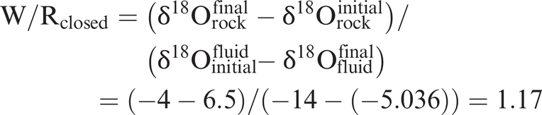
The geochemical effects of water–rock interaction can vary between two extremes. When the water–rock ratio is small, it is the δ18O in the rock that dominates the system and it is the fluid composition which is altered. On the other hand, when the water–rock ratio is large and the δ18O of the water dominates the system, then it is the δ18O value of the rock that is modified. Taylor (1974, 1977) derived mass balance equations from which the water–rock ratio may be calculated from δ18O values. For a closed system, from which no water is lost, the water–rock (W/R) ratio, integrated over the lifetime of the hydrothermal system, is:

This is the effective water–rock ratio which can differ from the actual water–rock ratio depending upon the efficiency of the exchange reaction. The initial value of the rock (δ18Orockinitial) is obtained from ‘normal’ values for the particular rock type (see Figure 7.1) or from an unaltered sample of the rock suite. The final value for the rock (δ18Orockfinal) is the measured value. The initial value for the fluid (δ18Oinitialfluid) is assumed (e.g., modern seawater) or in the case of meteoric water is calculated from D/H ratio of the alteration assemblage and the meteoric water equation. The composition of the final fluid (δ18Ofluidfinal) can be calculated from the mineralogy of the altered rock. This is sometimes done by using the approximation that δ18O plagioclase feldspar (An30) ~ δ18O rock, for feldspar is generally an abundant mineral in most rocks and exhibits the greatest rate of exchange between 18O and an external fluid phase. Provided that the temperature can be independently estimated, then the feldspar–water fractionation equation can be used to calculate the water composition (see the example below).
The equation for an open system in which the water makes only a single pass through the system is given by (Taylor, 1978) as
and the contrasting effects of open and closed systems on δ18O relative to the water–rock ratio are shown in Figure 7.10.
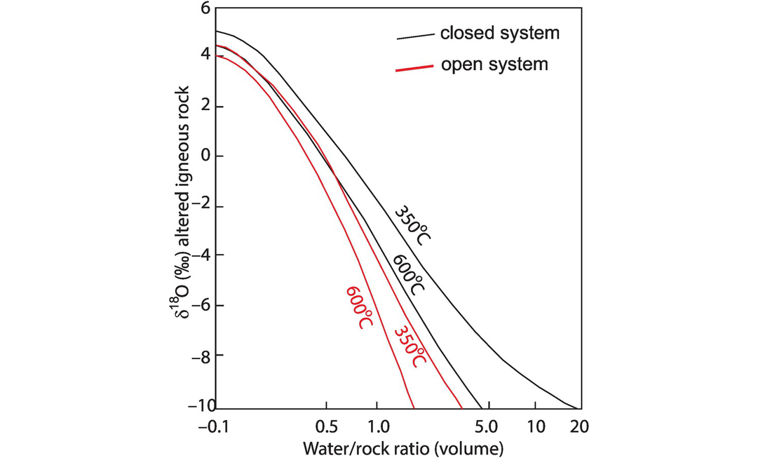
Plot of δ18O values in a hydrothermally altered rock calculated from the open-system water–rock ratio equation (Eq. 7.19) and the closed-system water–rock ratio equation (Eq. 7.18) (Taylor, 1974). The model assumes an initial δ18O value of +6.5 in the rock and an initial δ18O value of −14 in the water and curves are shown for 350oC and 600oC.
An example of how water–rock ratios may be calculated from oxygen isotope measurements is given in Box 7.5.
Data
Initial rock composition: δ18O = 6.5‰
Final rock composition: δ18O = −4.0‰
Initial fluid composition: δ18O = −14.0‰
Calculation of final fluid composition
The equation for plagioclase (An = 0.3) –water exchange from Table 7.2 is
at 500°C
Assuming δ18Ofsp ˜ δ18Owhole rock (final composition)
final fluid composition δ18O = −5.036‰
Water–rock ratio calculation
From the closed system equation (Eq. 7.18)
From the single-pass, open-system equation (Eq. 7.19)
Care should be taken in noting the units used for quantifying water–rock ratios, for both volume units and weight units are used. Both are shown in Figure 7.11. It is likely that any given hydrothermal system will behave some way between the two extremes of water-dominant and rock-dominant.
The effects on the isotopic composition of a hypothetical granodiorite pluton which crystallised under conditions of increasing water–rock ratio are shown on a δD versus δ18O plot in Figure 7.11, using the isotopic composition of biotite as a proxy for change in δD and the isotopic composition of feldspar as a proxy for change in δ18O (Taylor, 1978). At small water–rock ratios (up to 0.1 rock volumes) oxygen isotopic compositions are virtually unchanged, while δD values are reduced by about 100‰. As the water–rock ratio increases the δ18O value decreases rapidly at almost constant δD values. This is also illustrated in the study of Satir and Taubold (2001) on the Menderes gneiss complex in Turkey, who show that biotite is highly sensitive to the interaction of the gneiss with a very small amount of meteoric water and defines a trend of decreasing δD, while δ18O in feldspar remains constant as predicted by Taylor (1978).
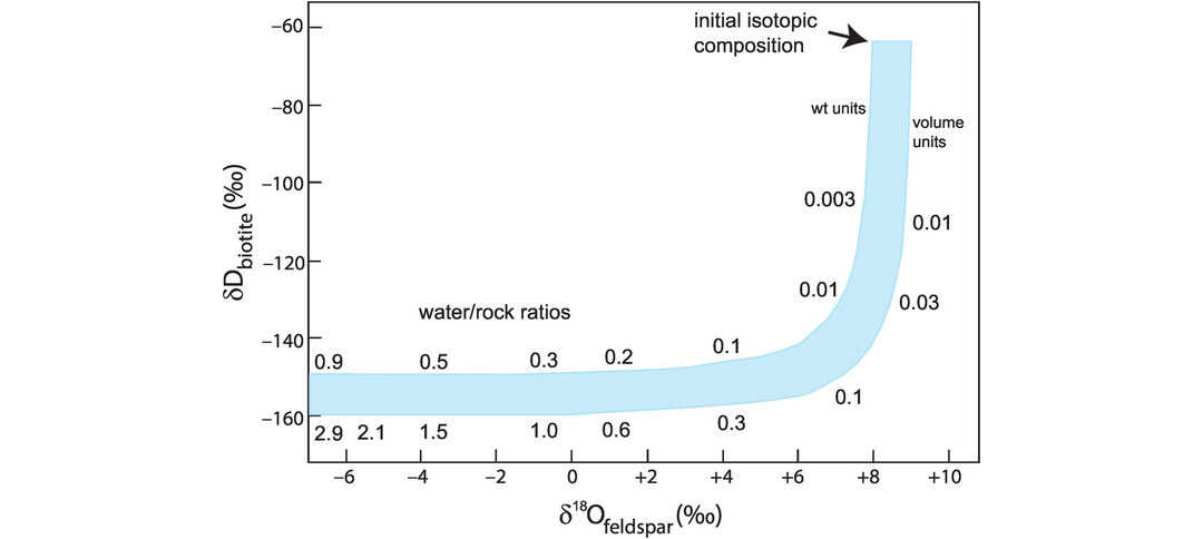
δD versus δ18O diagram showing the isotopic change in D in biotite and δ18O in feldspar in a granodiorite undergoing isotopic exchange with groundwater. The plotted curve shows the range of δD and δ18O values with changing water–rock ratios. The curve was calculated for an initial feldspar composition of δ18O = +8.0 to +9.0, biotite δD = −65.0 and the groundwater δD = −120, δ18O = −16. The fractionation of D between biotite and water at 400–450 oC is given by Δbiotite–water = −30 and −40; the fractionation of δ18O between feldspar and water at 400–450 oC is given Δfeldspar–water = 2.0. A small water–rock ratio has a dramatic effect on the isotopic composition of δD in biotite, whereas higher water–rock ratios affect both δD in biotite and δ18O in feldspar.
7.3.2.7 Examples of Water–Rock Interaction
There are many applications of the combined hydrogen–oxygen isotopic system to the study of water–rock interactions, and in this section a range of illustrative examples is given. As has already been shown, the sensitivity of hydrogen and oxygen isotopes to hydrothermal solutions means that they are excellent tools for detecting hydrothermal alteration in otherwise fresh rocks. Further, they may be used to identify the origin of the water and quantify its volume relative to the country rock.
(a) Interaction between igneous intrusions and groundwater. In a number of pioneering studies, Taylor and his co-workers showed that high-level igneous intrusions are frequently associated with hydrothermal convective systems (see review by Taylor, 1978). They found that the country rocks surrounding such intrusions are massively depleted in δ18O and D relative to ‘normal’ values and that the minerals in both the intrusion and the country rock are isotopically out of equilibrium with magmatic values. They concluded that the isotopic effects were due to the interaction between the magma and meteoric water and proposed that the intrusion acted as a heat engine which initiated a hydrothermal convection cell in the groundwater of the enclosing country rocks. Water–rock ratios were found to vary from ≪ 1.0 to about 7.0. These studies brought an important insight into attempts to establish the original isotopic composition of igneous rocks, for samples showing evidence of interaction with meteoric water may not preserve primary stable and radiogenic isotopic compositions.
More recently, the examination of oxygen isotopes in zircon is leading to a re-evaluation of some claims of high-level crustal interaction between igneous intrusions and meteoric water. For example, Taylor and Forester (1971) showed that the Western Redhills granites on the Island of Skye, Scotland, were characterised by low-δ18O phases, implying interaction with meteoric water during emplacement. However, subsequent zircon studies made by Gilliam and Valley (1998) show that these granites are low-δ18O magmas and that any interaction with groundwater may have taken place in their source rather than during emplacement.
(b) Interaction between ocean-floor basalt and seawater. A large number of studies have shown that the rocks of the ocean floor, now preserved as ophiolites, have undergone massive seawater-hydrothermal exchange and alteration. In a now-classic study of the Oman ophiolite, Gregory and Taylor (1981) showed that upper layers (dykes and lavas) of the ophiolite were enriched in δ18O, whereas the lower gabbro and peridotite layers were depleted in δ18O relative to average ocean crust (Figure 7.12). This cross-over of values, at about 250°C, is due to the temperature-dependent partitioning of oxygen isotopes between silicate minerals and seawater. Later studies showed a similar pattern of alteration in the Indian Ocean floor (Stakes et al., 1984), confirming the general applicability of the Gregory and Taylor model. Subsequent studies on hydrogen isotopes from amphibole in oceanic gabbros suggest that the hydrothermal fluid may also contain a component of magmatic water in addition to seawater (Stakes, 1991). These studies led to the important observation that the net exchange of δ18O between seawater and the ocean crust in the Oman ophiolite was zero (Gregory and Taylor, 1981), suggesting that the δ18O composition of seawater is buffered by the composition of the ocean floor, a view subsequently confirmed by Campbell et al. (1988).
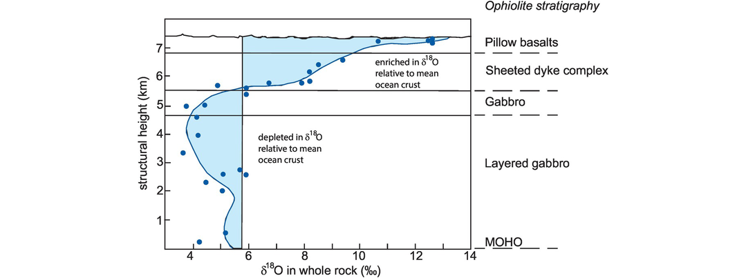
A whole-rock δ18O profile through the Oman ophiolite showing the relative enrichment and depletion in δ18O as a function of depth. Individual measurements are shown as solid blue circles.
(c) Water–rock interaction in metamorphic rocks. In metamorphic rocks oxygen isotopes are used to determine the patterns of fluid movement in a metamorphic sequence and establish the water–rock ratio. Fluid flow in metamorphic rocks may be pervasive, so that the fluid moves through pore spaces and establishes metamorphic equilibrium in the rocks (see, e.g., Chamberlain and Rumble, 1988), or may be channelised, migrating through cracks and fissures, in which case isotopic inhomogeneity may be preserved (see, e.g., Bottrell et al., 1990).
In addition, the combined study of hydrogen and oxygen isotopes can be used to determine the nature of the fluid originally in equilibrium with the metamorphic rock. Wickham and Taylor (1985) used this approach in their study of pelites in the French Pyrenees. They showed that the isotopic composition of muscovites had been homogenised through the influx of basinal formation waters which had exchanged their oxygen isotopes with the country rock.
(d) Water–rock interaction during the formation of hydrothermal ore deposits. An entire class of ore deposits is known to have formed from hydrothermal fluids. These fluids may be low or high temperature and associated with sedimentary, magmatic and, less commonly, metamorphic processes. Early studies such as that of Taylor (1974) were able to show the importance of oxygen and hydrogen isotopes in characterising these fluids and determining water–rock ratios. Indicative examples include the following:
Porphyry copper deposits. Qiu et al. (2016) use the composition of sericites plotted on a δD–δ18O diagram to show that the hydrothermal fluids in the Taiyangshan porphyry copper–molybdenum deposit of central China formed principally from magmatic fluids, with some small interaction with meteoric waters.
Kuroko-type massive sulphide deposits. A study of fluid inclusions in pyrite and chalcopyrite in Kuroko-type massive sulphide deposits from the Hokuroku district of Japan showed that their δD–δ18O compositions plot close to the composition of seawater which has experienced high-temperature isotopic exchange with the enclosing volcanic rocks (Ohmoto and Rye, 1974).
Mississippi Valley–type Pb–Zn deposits. Carbonate-hosted Pb–Zn sulphide deposits are thought to have formed in association with oilfield brines, although the origin of the brine is sometimes uncertain. A δD–δ18O study of fluid inclusions in sphalerite, fluorite and barite in the southern Appalachians showed that the brines originated as seawater but evolved to higher δ18O and lower δD by mixing with water that has reacted with organic matter (Kesler et al., 1997).
7.3.3 Carbon Isotopes
Carbon occurs in nature in its oxidised form (CO2, carbonates and bicarbonates), as reduced carbon (SiC, methane and organic carbon) and as the native element in diamond and graphite. Further, carbon is found throughout the whole solid Earth system from the core to the crust as well as in the oceans, atmosphere and biosphere.
There are two isotopes of carbon, 12C and 13C; isotope ratios are measured as 13C/12C and expressed as δ13C‰ (Eq. 7.20). In natural systems carbon isotope compositions vary over 100‰. The essential data for stable isotopes of carbon are given in Box 7.6. Figure 7.13 shows the variation in δ13C in the major Earth reservoirs, and the main fractionations and their mechanisms in the global carbon cycle are shown in Figure 7.14 (after Suarez et al., 2019).
Stable isotopes and abundances
14C is a short-lived radioactive isotope with a half-life of 5730 years, produced by the action of cosmic rays on 14N in the atmosphere. It decays to 14N.
Measured isotope ratio
Standard
VPDB: Vienna Peedee belemnite from the Cretaceous Peedee formation of South Carolina, USA. This standard is used because its 13C and 18O values are close to those of average marine limestone. The original material of the PDB standard is now exhausted and current standard materials are a carbonatite NBS-18 and marine limestone NBS-19.
Mantle value
Bulk silicate Earth
Variations in nature
See Figures 7.13 and 7.14.
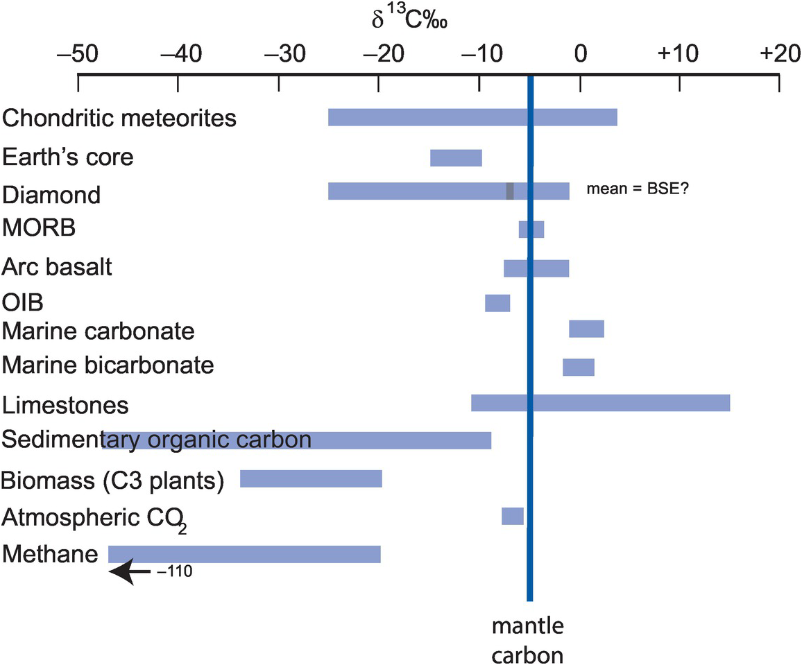
Variations in δ13C in the major Earth carbon reservoirs relative to the Earth’s mantle. (Data sources in the text)
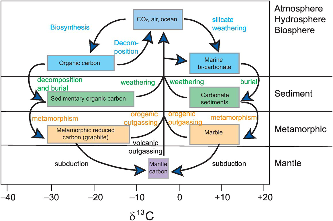
The major Earth carbon reservoirs and the processes that control carbon isotope fractionations between them.
It is important to recognise the complexities of the Earth’s carbon cycle (Figure 7.14) inasmuch as it includes both the short-term surficial carbon cycle which operates on a time scale of a maximum of 10,000 years and the long-term deep-Earth carbon cycle which operates on a time scale of Ga. The short-term carbon cycle is focussed on the terrestrial biosphere and is concerned with exchanges between the biosphere, the atmosphere and the oceans. The deep-Earth carbon cycle is focussed on the emission of CO2 from volcanic sources; carbon drawdown through weathering, photosynthesis and carbonate formation; and the return of these materials to the mantle through subduction. Current estimates suggest that the present-day fluxes of CO2 into the mantle broadly match the amount released, implying that at the present time the mantle is at a steady state with respect to carbon (Rollinson, 2007). In this section we explore the role that carbon isotopes play in elucidating the balances in and between the surfical and deep-Earth carbon cycles.
Carbon isotopes are measured as CO2 gas, and precision is normally better than 0.1‰. CO2 is liberated from carbonates with >103‰ phosphoric acid or by thermal decomposition. Organic compounds are normally oxidised to CO2 at very high temperatures in a stream of oxygen or with an oxidising agent such as CuO. In situ measurements made by ion probe using secondary ion mass spectrometry (SIMS) use a focused 133Cs+ primary beam. The impact of the 133Cs+ atoms sputters ions off the sample surface. Sputtered ions are accelerated in the mass spectrometer and are sorted by their mass/charge ratio before reaching an array of Faraday cup and electron multiplier detectors. Analyses are made using an appropriate running standard (Denny et al., 2020).
7.3.3.1 Controls on the Fractionation of Carbon Isotopes
The fractionation of carbon isotopes is controlled by both equilibrium and kinetic processes. Equilibrium fractionation factors for carbon isotopes for a range of carbon-bearing species relative to CO2 are shown in Figure 7.15. The fractionation factors (α) were obtained from both theoretical and empirical studies and are discussed by Chacko et al., 2001. It can be seen from the carbonate curves in Figure 7.15 that at relatively low temperatures carbonate precipitated from CO2 is enriched in 13C, whereas at higher temperatures the carbonate is depleted in 13C. At very high temperatures the fractionation factors converge and so at mantle temperatures (~1000°C) carbon isotope fractionation between coexisting C-bearing species is small and less than 4‰ (Bottinga, 1969). Additional high-temperature fractionation curves include those for carbon-bearing species relative to carbides (Horita and Polyakov, 2015), and for atomic carbon (Deines, 2002). Fractionation factors between diamond and carbonate and diamond and carbon dioxide are given in Smit et al. (2016). At lower temperatures the fractionation of carbon isotopes between carbonates and organic carbon is such that δ13C values in organic carbon are on average 25‰ lower than in co-existing carbonate carbon (see Figure 7.16).
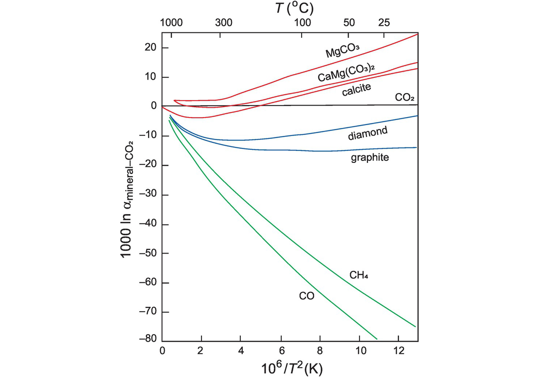
Fractionation factors shown as 1000 ln α for carbon species relative to CO2 versus temperature – shown as degrees C on the top axis and as 106/T2 Kelvin on the lower axis.
In addition to mineral–CO2 carbon isotope fractionation, carbon isotopes are also fractionated during volcanic degassing. 13CO2 versus 12CO2 fractionation during degassing depends upon the fractionation factor between dissolved CO2 in the melt and CO2 vapour. These fractionation factors are between +2.3‰ and +4.6‰ such that there is lower δ13C in the melt–CO2 relative to the exsolved gas phase. The processes are summarised in Barry et al. (2014), who show that they include closed system, batch equilibrium degassing in which vesicles stay in contact with the melt and open system degassing when vesicles form in equilibrium with the surrounding melt but are removed during degassing. Similar principles apply to devolatisation reactions in metamorphic rocks, and Valley (1986) has calculated the differential fractionation of carbon isotopes during batch de-volatilisation and Rayleigh (fractional) devolatisation (Figure 7.18b) in metamorphic systems.
Kinetic fractionation of carbon isotopes is important in biological processes such as the fixing of CO2 as organic carbon and the evolution of methane during the anaerobic fermentation of organic matter during diagenesis. In these cases fractionation is controlled by the greater readiness of the lighter isotope to react, and reactions can be identified which relate to specific biogenic pathways. For example, the process of photosynthesis in green plants and algae using the enzyme rubisco may lead to the fractionation of δ13C of −30‰, although in detail there several different pathways and more than one version of rubisco. Similarly, the process of methanogenesis, that is, the production of methane through the reduction of CO2 by hydrogen in methanothermobacteria, may lead to δ13C fractionations in the range −22 to −58. Where the reaction involves both carbon and oxygen, the kinetic effect will influence the isotopes of both elements in a similar way, and a correlation between δ18O and δ13C is expected.
7.3.3.2 Carbon Isotopes in Meteorites
Carbon is present in chondritic meteorites in the form of organic compounds, carbonates, carbides, graphite and diamond. Grady and Wright (2003) estimate that the bulk δ13C in the different chondritic meteorite groups ranges from −25 to +4‰ (Figure 7.13), although in detail the composition of individual carbon-bearing molecules and mineral species is much more variable (Simkus et al., 2019). The solar value for δ13C, based upon the bulk composition of nanodiamonds in the Allende meteorite, is δ13C = +8 ± 35‰ (Lewis et al., 2018).
The presence of dissolved carbon together with graphite and carbide inclusions in iron meteorites strongly suggests that the Earth’s metallic core sequestered carbon during core–mantle differentiation. Experimental and modelling studies indicate that this process would preferentially partition the lighter isotope into the metallic phase (Satish-Kumar et al., 2011; Horita and Polyakov, 2015). Although the precise δ13C value of the core is not known, Horita and Polyakov (2015) estimate it to be in the range −10 to −15. Nevertheless, currently there is much uncertainty in this field, with the result that it is not possible to use a chondritic model for the isotopic composition of the Earth, and the carbon isotopic value for the bulk Earth is unknown (Mikhail and Furi, 2019).
7.3.3.3 Carbon Isotopes in the Mantle
Isotopic measurements on mid-ocean ridge basalts, carbonatites, kimberlite xenoliths and some diamonds define a mean mantle value of δ13C ~ −5.0‰ (Deines, 2002), although some authors place an error of ± 3‰ on this value (Cartigny, 2005). This mantle range probably represents an isotopic homogenisation event during the early differentiation of the Earth. The more varied isotopic composition of fluids in the sub-continental lithospheric mantle is revealed by the carbon isotope composition of diamonds. These show a wide range of δ13C values from ~−3.3 to −26 (Deines, 2002; Deines et al., 2009; Mikhail and Furi, 2019), and there is geochemical evidence to support the view that the isotopically light carbon was derived from subducted organic carbon (Mikhail and Furi, 2019). The mean δ13C value of all diamonds worldwide is −7.2‰, and since these include diamonds from the lower mantle Horita and Polyakov (2015) suggest that this value might represent that of the bulk silicate Earth.
7.3.3.4 Carbon Isotopes in Igneous Rocks
CO2 behaves highly incompatibly during mantle melting and so partitions almost entirely into the melt phase (Dasgupta and Hirschmann, 2010). This means that the CO2 content of magmas is a function of the carbon content of the mantle source and the degree of partial melting (Black and Gibson, 2019). Measuring the original CO2 content of volcanic rocks is difficult because of the process of degassing, although estimates can be made from trace element ratios such as CO2/Nb and CO2/Ba, for Nb and Ba have a similar incompatible element behaviour to that of CO2.
Marty et al. (1999) found that the carbon isotope composition of mid-ocean ridge basalts from a range of locations around the world results in a near constant ratio, which is within the typical mantle range, of δ13C = −5.2 ± 0.7‰. This value can be taken as representative of the depleted mantle. The carbon isotope composition of arc basalts is slightly lighter than that of MORB and is thought to be controlled by a mixture of mantle carbon and carbon derived from subducted carbonate sediments and is in the range δ13C = −8 to −2‰ (Eguchi et al., 2020). The carbon isotope composition of ocean-island basalts is also lighter than that of MORB and arc basalts and is in the range δ13C = −9 to −7‰ (summarised in Eguchi et al., 2020). These low values may reflect the presence of subducted organic carbon in the mantle source. Even lower values have been recorded but these are thought to reflect carbon isotope fractionation during volcanic degassing.
Carbon from degassed volcanic rocks as found in hydrothermal volcanic fluids is much more variable in composition than that in the melts themselves. This is in part due to fractionation during degassing and carbonate precipitation, but also as result of mixing with crustal rocks. Barry et al. (2014) report geothermal fluids from Iceland with δ13C in the range −18.8 to +4.6 (mean −4.0 ± 3.7), thought to be the result of fractionation during degassing and carbonate precipitation. However, they calculate that the pre-eruptive value is δ13C = −2.5 ± 1.1, much closer to that of the depleted mantle. Volcanic fluids from Tanzania have δ13C in the range −2.3 to −6.5 (mean −3.1 ± 1.9), also close to mantle values, but in this case a δ13C versus CO2/3He plot reveals that these gases are mixtures of mantle carbon, carbon derived from limestones and an organic source (Barry et al., 2013).
7.3.3.5 Carbon Isotopes in Carbon-Bearing Sediments
The carbon isotope ratio of marine carbonates and of organic matter in the oceans is controlled by the addition of carbon to the ocean–atmosphere system. In the modern Earth a balance is maintained between the volcanic outgassing of mid-ocean ridge and arc lavas and the removal of carbon through silicate weathering and the burial of organic carbon in sediments.
Modern seawater has, by definition, a δ13C value close to 0‰ and marine carbonates therefore have values close to this composition. This means that ancient limestones can be used as a proxy for the composition of seawater in the past. Figure 7.16 shows the variation in δ13C in marine carbonates and marine organic carbon over geological time, indicating that there have been some major departures from modern values during Earth history. Possible mechanisms to explain these variations include episodes of extreme volcanic outgassing such as those associated with the formation of large igneous provinces (Black and Gibson, 2019). Alternatively, it has been suggested that an increase in the rate of burial of organic sediments in the oceans leads to the preferential removal of isotopically light carbon (Krissansen-Totton et al., 2015; Eguchi et al., 2020) and produces a δ13C spike. A change in the rate of the burial of organic carbon may, in turn, be related to levels of oxygen in the Earth’s atmosphere and therefore linked to the rise of photosynthesising organisms.
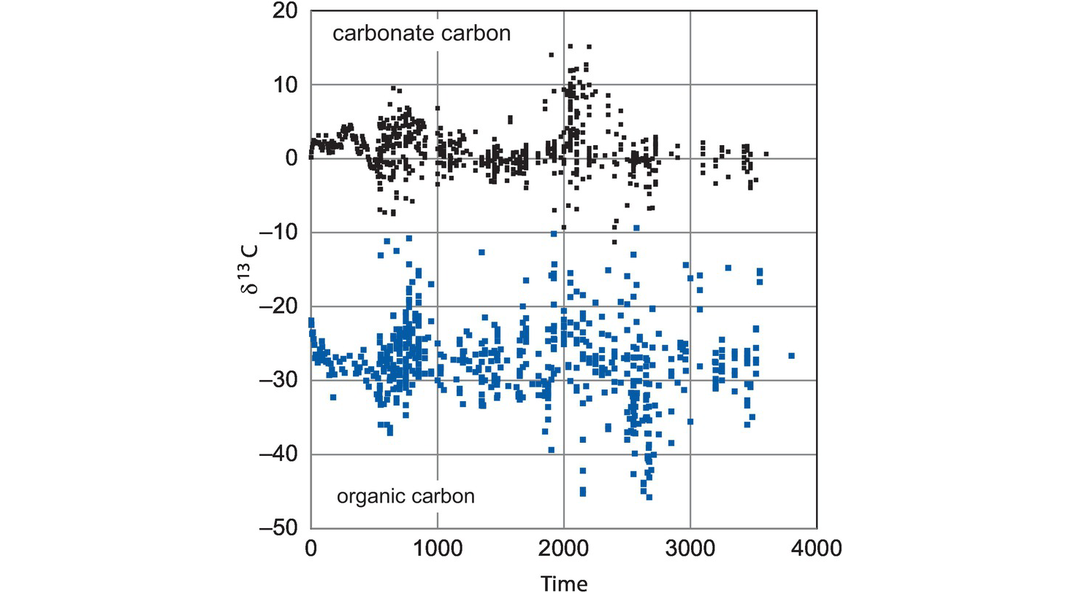
δ13C measurements in carbonate rocks since ~3500 Ma, and δ13C measurements in organic carbon since ~3800 Ma.
In addition to the global δ13C curves discussed above, high-resolution δ13C measurements can be made on specific stratigraphic sequences and used to illuminate particular geological processes. For example, Kämpf et al. (2020) use δ13C in modern varved lake sediments as a proxy for flood events.
7.3.3.6 Biologically Derived (Organic) Carbon
The conversion of inorganic carbon through a CO2-fixing mechanism into living, organic carbon entails the preferential concentration of the light 12C isotope in organic carbon. This process is chiefly controlled by reaction kinetics which favour the light isotope. At a global level the net effect of this fractionation is that relative to mantle-derived carbon (δ13C ~ −5‰) there are two complementary reservoirs. Biological materials are strongly depleted in δ13C (−20 to −30‰), whereas seawater and marine carbonates (δ13C ~ 0‰) are slightly enriched (Figure 7.16). At a more detailed level the knowledge of specific fractionations in biological materials is now used in the carbon isotope fingerprinting of different plant groups and in the identification of particular biological and climatic processes (see, e.g., Kohn, 2010).
Methane is the most depleted of all carbon compounds and is commonly formed in nature either by the anaerobic fermentation of organic matter or by the thermal degradation of petroleum or kerogen at temperatures greater than 100°C. Methane of biological origin has a range of δ13C values from about −30‰ to −110‰, whereas abiotic methane has δ13C values between −50 and +10‰. Reeves and Fiebig (2020) helpfully classify methane of microbial and abiotic origin according to its δD and δ13C composition (Figure 7.17).
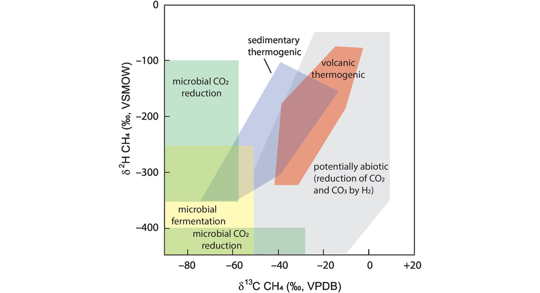
δD (δ2H) versus δ13C plot in methane showing the different types of microbial and abiotic methane.
7.3.3.7 Carbon Isotopes and the Search for Early Life on Earth.
Schidlowski (1988) showed how the study of carbon isotopes can be used to trace ancient biological activity through the geological record. The argument is based upon the observation that isotopically light, organic carbon and isotopically heavy carbonates are complementary reservoirs which have originated from the biological fractionation of mantle carbon. Both reservoirs therefore are responsive to changes in the level of biological activity. Schidlowski (1988) showed that there is very little change in the degree of fractionation between the two reservoirs from the present day to the earliest part of the geological record at 3.8 Ga and argued for the constancy of biological activity since 3.8 Ga and presence of CO2-fixing organisms since this time. Subsequent studies such as that of Rosing (1999) have validated the early work of Schidlowski (1988) and show that the geological record preserves very low δ13C organic carbon signatures in rocks as old as 3.7 Ga (Figure 7.16). There are, however, problems in uniquely identifying biogenic signatures in the ancient sedimentary record, for there is an overlap in the degree of carbon isotope fractionation between biogenic and abiotic processes. Horita (2005) showed that abiotic reactions can produce carbon isotope fractionations that are as large as those driven by biogenic processes, and these will produce a similar degree of fractionation to that created by methanogenic bacteria.
7.3.3.8 Carbon Isotopes in Crustal Fluids
Crustal CO2-bearing fluids can be subdivided into those which are present during metamorphism, fluids related to mineralising processes and other forms of fluid–rock interaction.
(a) Metamorphic fluids. The principal controls on carbon isotope fractionation during metamorphism are illustrated in Figure 7.14, and the relevant physical fractionation processes were reviewed by Valley (1986). The decarbonation of a marine limestone during metamorphism leads to lighter (more negative) δ13C in calcite (Nabelek et al., 1984; Epstein et al., 2020), and the CO2 released is correspondingly heavier in δ13C. The metamorphism of biogenic, non-carbonate carbon, on the other hand, leads to a loss of methane and heavier (less negative) δ13C values in the residual graphite. However, this simple guide is not always applicable, for metamorphic graphite may also be produced by the mixing of carbon-bearing fluids as in the case of hydrothermal vein graphites in the high-grade gneisses of New Hampshire (Rumble and Hoering, 1986) and in pelites from the Ivrea zone (Baker, 1988). Studies of the fractionation of carbon isotopes during subduction zone metamorphism may be used to refine models of the global carbon cycle and assess the fate of carbon-bearing sediments during the subduction process and the associated release of CO2 (Piccoli et al., 2016; Epstein, 2020).
(b) CO2 in gold-mineralising fluids. Carbonate minerals precipitated in association with Archean lode gold deposits are thought to result from the CO2-rich nature of the auriferous fluids and as such are potentially an indicator of the source of the gold-bearing solutions (Groves et al., 1988). Early studies found that the mean δ13C value of calcite carbon was between −3 and −4‰ and concluded that the CO2-rich fluids were externally derived and of mantle origin (Burrows et al., 1986). However, in a review of orogenic gold deposits, Goldfarb and Groves (2015) show that the carbon isotope compositions of associated calcites are extremely variable and range from δ13C = +2 to −30, implying multiple local sources and carbon isotope fractionations during deposition. They conclude that the variability in δ13C in ore fluids and for ore-related carbonates in orogenic gold deposits ‘makes it very difficult to use such data to clearly define a carbon source for the ore-forming fluids’. A better approach therefore is to combine carbon isotopes measurements with measurements from another stable isotope system as discussed in Section 7.3.3.9.
(c) CO2 fluid–rock interaction. The principles of fluid–rock interaction were discussed in the section on water–rock interaction (Section 7.3.2.6). When the fluid–rock ratio is small, the δ13C in the rock dominates the system and the composition of the fluid is changed, whereas when the fluid–rock ratio is large and the δ13C of the CO2–fluid dominates, it is the δ13C value of the rock that is modified. Mass balance calculations require a knowledge of the initial δ13C values for the carbonate and the fluid, the proportions of the carbon-bearing species and the fractionation factors for 13C between CO2 and the carbon-bearing species (see Section 7.3.3.1). The shift in δ13C from the original to that measured in calcite and/or graphite is used to calculate the extent of fluid–rock interaction. Examples are given by Baker (1988) and Skelton (2015). Baker (1988) found very low fluid–rock ratios in the amphibolite and granulite facies rocks of the Ivrea zone, whereas Skelton (2015) found fluid–rock ratios of more than 30:1 in carbonate rocks from Islay, Scotland.
7.3.3.9 Combined Oxygen and Carbon Isotope Studies of Carbonates: δ18O–δ13C Plots
A combined study of carbon and oxygen isotopes in carbonates is a powerful means of distinguishing between carbonates of different origins and for understanding processes in carbonate rocks. On a δ18O–δ13C diagram (Figure 7.18) oxygen isotope compositions are plotted relative to the VSMOW standard and carbon isotopes relative to VPDB. We focus on the signatures of limestone diagenesis, hydrothermal calcite and metamorphic rocks.
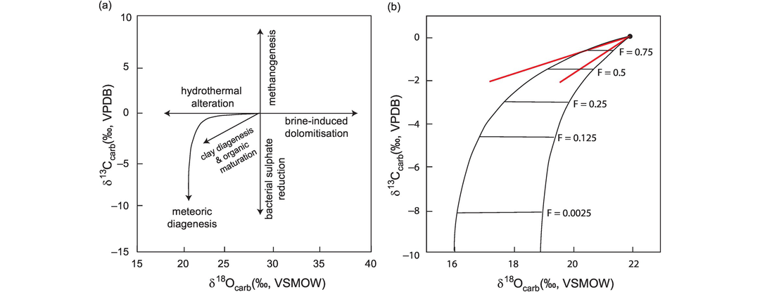
Coupled δ18O–δ13C diagrams. (a) The effects of a range of diagenetic process on the isotopic fractionation of carbon and oxygen isotopes in carbonate sediments (after Reis et al., 2019; with permission from Elsevier). (b) δ18O–δ13C trends which result from the devolatilisation of a calc silicate rock during batch fractionation (red lines) and Rayleigh fractionation (black lines). The curves are calculated for two values of oxygen fractionation factor (α18O CO2–rock = 1.012 to 1.006) and α13CCO2–rock = 1.0022. Initial values are δ18O = +22 and δ13C = 0. F values are the mole fraction of carbon which remains in the rock after fractionation.
(a) Limestone diagenesis. The δ18O–δ13C diagram is particularly useful in understanding the processes of limestone diagenesis and has the potential to distinguish between marine, organic and methane-related carbon (Coleman and Raiswell, 1981). Oxygen isotopes in sedimentary carbonates can be used to determine the origin of the fluids in equilibrium with the carbonates and can also provide an estimate of the temperature of carbonate formation using the Epstein et al. (1953) thermometer (Eq. 7.13), although care should be taken to establish chemical equilibrium (McConnaughey, 1989). A summary of the fractionations which can take place in carbon and oxygen isotopes in carbonate rocks during deposition, burial and exhumation is given in Figure 7.18a (after Reis et al., 2019).
A fruitful approach to understanding limestone lithification is through the isotopic analysis of the different generations of carbonate produced during this process. This allows the construction of an evolutionary pathway on a δ18O–δ13C diagram and shows the isotopic history of the rock. Denny et al. (2020) show how combined ion-probe measurements of δ18O and δ13C on zoned diagenetic carbonates can be used to monitor changing fluid compositions and temperatures in different parts of the Williston basin in the northern United States.
(b) Hydrothermal calcite. Hydrothermal calcites formed by water–rock interaction at a mid-ocean ridge show a wide range of compositions on a δ18O–δ13C plot, chiefly as a function of differing water–rock ratios (Stakes and O’Neill, 1982). At one extreme, calcite in a greenstone breccia has mantle-like δ13C values and formed in a rock-dominated environment (low water–rock ratio) at high temperature (145–170°C). In contrast, low-temperature vein calcites have seawater δ13C values and represent a large volume of seawater interacting with the host basalts.
Calcites associated with Mississippi Valley–type lead–zinc mineralisation in Carboniferous limestone in Illinois show a marked decrease in δ13C during their growth coupled with only a small decrease in δ18O. These changes indicate that early calcites were very similar to the composition of carbonates in the limestone, while late in the evolution of the hydrothermal system, fluids associated with the degradation of organic carbon become important (Richardson et al., 1988).
In carbonaceous chondrites hydrothermal calcite may form during the planetary weathering which takes place in the formation of planetesimals. In this case a plot of δ18O–δ13C allows an estimate to be made of their temperature of formation, the composition of the gas mixture from which they were precipitated and subsequent processes of dissolution and reprecipitation (Telus et al., 2019).
(c) Metamorphic rocks. Valley (1986) showed how the composition of δ18O and δ13C varies between batch and Rayleigh fractionation during the metamorphism of carbonate rocks. Both types of fractionation lead to a similar reduction in δ18O, but δ13C values are fractionated to much lighter values during Rayleigh fractionation (Figure 7.18b). Coupled δ18O and δ13C trends for many examples of contact metamorphism show a strong coupled decrease in δ18O and δ13C with increasing grade of metamorphism. A similar pattern is found in the subduction zone metamorphism of marine carbonates in the western Alps (Epstein et al., 2020).
7.3.3.10 Carbon Isotope Thermometry
Inspection of Figure 7.15 shows that the fractionation of 13C between carbon-bearing phases is strongly temperature-dependent. Following Bottinga (1969), a number of workers have shown how these fractionations may be used as thermometers. Kueter et al. (2019) provide an experimental calibration of the partition of carbon isotopes between carbonate phases and graphite and diamond and show how this can be used as a geothermometer. Their experiments were conducted at high temperatures (1200–1500°C) on carbonate melt and graphite and extended to lower temperatures using natural partitioning data in metamorphic rocks. They propose the following thermometer:
in which temperature T is in K. This thermometer is calibrated in the range 610–1500°C and is applicable to carbonates which are in the solid and molten state, meaning that the thermometer is applicable to metamorphic and magmatic carbonate–graphite pairs. At mantle temperatures the fractionation of carbon isotopes between calcite and Mg–calcite and between graphite and diamond is very small, of the order of 0.1‰, which means that the carbonate–graphite thermometer may also be applied to magnesian carbonates and diamond.
In an older application, the carbon isotope composition of CO2 in fluid inclusions and that of coexisting graphite was used as a thermometer. The exchange was calibrated by Bottinga (1969) and the method was used by Jackson et al. (1988), who obtained equilibration temperatures close to the peak of metamorphism from CO2-rich inclusions in quartz and graphite in granulite facies gneisses from South India.
7.3.4 Sulphur Isotopes
Naturally occurring sulphur-bearing species include native sulphur, the sulphate and sulphide minerals, gaseous H2S and SO2 and a range of oxidised and reduced sulphur ions in solution. A summary of the isotopic compositions of some major Earth reservoirs and rock types is given in Figure 7.19.
Sulphur has four stable isotopes – 32S, 33S, 34S and 36S – and three different stable isotope ratios can be measured. Until the year 2000 most sulphur isotope studies reported only values for δ34S because the two isotopes involved (34S and 32S) are more abundant (see Box 7.7) and relatively straightforward to measure. The lower abundances of 33S and 36S had meant that their measurement was more difficult, although with technological improvements and the discovery that these isotope ratios have geological significance they are now also frequently measured.
Stable isotopes and abundances
Measured isotope ratios
Delta notation (see Section 7.2.4)
Standards
Troilite (FeS) from the Canon Diablo iron meteorite (CDT)
V-CDT is based on the reference material IAEA-S-1 (Ag2S)
On the CDT scale ISEA-S1 has the composition δ33S = −0.091‰, δ34S = −0.401‰, δ36S = −1.558‰, Δ33S = 0.116‰, Δ36S = −0.796‰ (Dottin et al., 2020)
Mantle value (depleted upper mantle)
Variations in nature
See Figure 7.19.
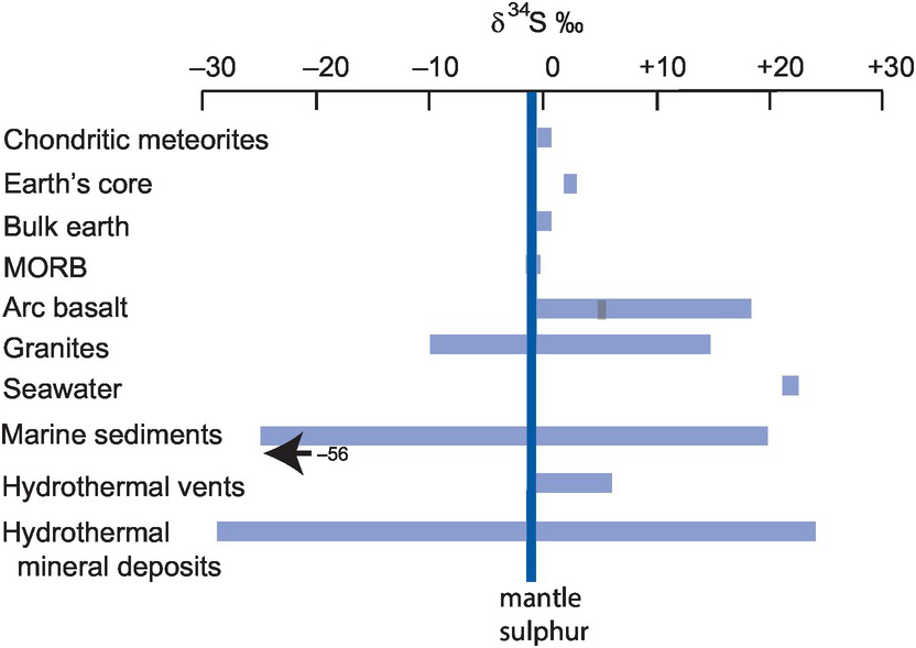
Variations in δ34S (expressed relative to V-CDT) in major Earth reservoirs and rock types relative to the sulphur isotope composition of the Earth’s mantle.
Given that three different sulphur ratios can be determined, it is possible to discriminate between mass-dependent and mass-independent fractionation in the sulphur isotope system (see Section 7.2.4). Mass-dependent fractionation is based upon the assumption that the fractionation between the different isotopes is dependent upon their mass differences and so, for example, the fractionation of δ33S ~ 0.5 ∗ δ34S. The actual value is determined from the slope of a plot of terrestrial sulphide and sulphate values for the two isotope ratios and is found to be 0.515 for equilibrium fractionation (Box 7.7). Mass-independent fractionation represents deviation from the mass-dependent fractionation line and implies that a different set of processes is operating. Mass-independent fractionation is quantified using the Δ notation and the term Δ33S represents the fractionation of δ33S relative to δ34S. In the modern Earth Δ33S is zero, but in the early history of the Earth both positive and negative deviations have been recorded (Farquhar and Wing, 2003). The Δ notation is calculated following Eqs. 7.8 and 7.9 (Box 7.7) following Farquhar and Wing (2003). A slightly different calculation is given by Mishima et al. (2017), although the two definitions are almost identical where variations in δ34S are less than ± 10‰.
Older sulphur isotope measurements were based upon the analysis of SO2 gas; precision during mass spectrometry was ~0.02‰ and accuracy about 0.10‰. Modern analyses, however, require very high precision in order to measure the lower abundance isotope ratios δ33S and δ36S, and so sulphur is now converted into SF6 gas. This is to be preferred because fluorine has only one isotope and so the use of SF6 reduces the number possible mass interferences from the method where multiple oxygen isotopes were involved (Ono et al., 2006). The gas chromatography–mass spectrometry fluorination method of Ono et al. (2006) can also be applied to the in situ laser ablation of samples, using a KrF laser. In this case the spatial resolution is of the order of ~150 μm in diameter.
Multiple sulphur isotopes (32S, 33S, 34S) can be also analysed by the ion microprobe (SIMS) using simultaneous multicollection methods. The sulphur may be analysed as either positive or negative ions, although negative secondary ions give a greater yield and so typically a 133Cs+ primary beam is used (Whitehouse et al., 2005). Precision for Δ33S is between 0.2 and 0.3‰ and the spatial resolution is of the order of ~25 μm in diameter. Hauri et al. (2016) describe the high-precision analysis of sulphur isotopes using a nanoSIMS in which the spatial resolution is in the order of ~15 μm.
The primary input into the Earth’s sulphur cycle comes from volcanic sulphur dioxide which in the Earth’s stratosphere converts to sulphate aerosols. This returns to the Earth’s surface through precipitation, weathering and riverine input into the oceans. Sulphur-rich fluids also enter the oceans through the outgassing of submarine magmas at mid-ocean ridges and their related hydrothermal systems. Sulphur is removed from the oceans primarily through pyrite precipitation, principally driven by sulphate-reducing bacteria, and to a lesser degree through sulphate–evaporite deposits. Sedimentary pyrite and sulphate are then returned either to the weathering cycle as a result of tectonic uplift or to the mantle through subduction.
These processes include a range of sulphur isotope fractionations (see Section 7.3.4.2), which give rise to three isotopically distinct sulphur isotope reservoirs. These are the following:
(1) Mantle-derived sulphur with δ34S values in the range −1 to −2‰
(2) Seawater sulphur with δ34S today = +21‰, although this value has varied in the past
(3) Strongly reduced (sedimentary) sulphur with large negative δ34S values.
Sulphur isotope studies today play an important role in unravelling the Earth’s global sulphur cycle, both in the present and over geological time, in particular, monitoring major changes during the evolution of the Earth’s atmosphere and oceans and the development of life on Earth. In addition, sulphur isotopes play a major role as geological tracers and are used to identify the sources of sulphide and sulphate in a variety of geological environments.
7.3.4.1 The Distribution of Sulphur Isotopes in Nature
Unequilibrated chondritic meteorites have a narrow range of δ34S and Δ33S values, close to those of the sulphur isotope standard, the mineral troilite in the Canyon Diablo iron meteorite (CDT). Primitive chondrites have δ34S values averaging 0.0 ± 0.3‰ and average Δ33S indistinguishable from that of CDT. Ordinary chondrites have δ34S = +0.04 ± 0.10‰ and are thought to represent the bulk Earth value. Melting experiments show that the Earth’s core was enriched in 34S; this sulphur would have been dissolved in the alloys of the Earth’s core, leading the residual mantle to be 34S-deficient relative to the bulk Earth (Labidi and Cartigny, 2016, and references therein).
It has been proposed that minimal isotope fractionation takes place during mantle melting, and so estimates of the sulphur isotopic composition of the depleted upper mantle can be made from measurements on mid-ocean ridge basalts (Labidi and Cartigny, 2016). δ34S values for MORB glasses range from −0.68 ± 0.09 to −1.28 ±0.33‰ and an average Δ33S = +0.008 ±0.006‰, the latter indistinguishable from CDT and bulk chondrites. Slightly higher values are reported for plume basalts with δ34S in the range 0 to +3.0‰ (Dottin et al., 2020), which may indicate the deep recycling of 34S-enriched materials.
Arc volcanic rocks are derived from a mantle source which is enriched in δ34S relative to MORB and OIB sources. Globally, they show a wide range of sulphur isotope values with δ34S between −2.0 and +18.0‰, although individual arcs have a smaller range. A global average for arc volcanic rocks is δ34S = +5.3 ± 4.0‰ (de Hoog et al., 2001). Li et al. (2020) have argued that the positive δ34S signature of the sub-arc mantle cannot be derived from slab-derived fluids in a subduction zone and that subducted slabs return a negative δ34S contribution of ~−3.7‰ to the deep mantle.
Crustal rocks show also show a wide range of δ34S values. Bulk rock sulphur isotope measurements on granitoids range in composition from δ34S =~ −10 to +15‰ (see, e.g., Coleman, 1977; Yang and Lentz, 2010). This variation reflects the diverse protoliths involved in granitoid genesis and varying degrees of interaction between granitic melts and their host rocks.
The average δ34S value for sulphate in modern seawater is 21.24 ± 0.88‰ and the average value for Δ33S value is +0.05 ± 0.014‰. Riverine δ34S input varies between 5 and 15‰ depending upon the weathering source (Tostevin et al., 2014). Present-day marine sulphate evaporites are enriched in δ34S by between 1 and 2‰ relative to seawater, a relationship exploited by Claypool et al. (1980) and Crockford et al. (2019) to determine the δ34S value of ancient seawater. Crockford et al. (2019) summarise the changes in δ34S and Δ33S in sedimentary sulphate since the Archaean and show from evaporite data that there were major positive and negative excursions relative to modern values over geological time. δ34S in other modern marine sediments has an extensive range with values from +20‰, reflecting the composition of seawater, down to −56‰, the product of bacterial sulphate reduction to form pyrite.
δ34S in modern hydrothermal vent chimneys from mid-ocean-ridge settings have bulk rock values in the range −1.0 to 6.0‰. This range of values reflects the mixing of MORB-derived sulphur with seawater sulphate (Butler et al., 1998). Sulphides in hydrothermal mineral deposits of volcanogenic and sedimentary origin show a very wide range of δ34S values, reflecting the multiple sources of the sulphur in these environments. Compare, for example, measurements for a porphyry Mo deposit (δ34S = 1.5 to 3.8‰; Han et al., 2018) with findings for a shear-hosted gold deposit (δ34S = −12.6 to +23.5‰; Godefroy-Rodríguez et al., 2020). In addition, recent in situ sulphide analyses show a huge variation in the δ34S values of the different sulphide species within an individual mineral deposit (Li et al., 2019).
7.3.4.2 Controls on the Fractionation of Sulphur Isotopes
Inspection of Figure 7.19 shows that crustal rocks and sediments have a wide range of δ34S values. These ranges of values indicate either fractionation or mixing processes. In this section we consider the main fractionation mechanisms in igneous and sedimentary rocks.
(a) Sulphur isotope fractionation in igneous rocks. Magmas may be rich in either SO2 or H2S. This is a function of the oxidation state of the melt and in part this depends upon pressure. Typically, high pressure favours H2S, whereas at low pressures SO2 is the dominant species (Rye, 2005). The fractionations of sulphur isotopes during igneous processes are relatively small. For example, Labidi and Cartigny (2016) in their investigation of mid-ocean ridge basalts found that there is ‘negligible sulfur isotope fractionation during partial melting’ of the Earth’s mantle. This is an important observation for it means that the sulphur isotope composition of basaltic rocks can be taken to reflect the isotopic composition of their source.
Isotope fractionation during magmatic differentiation is more complex because a number of different processes may be operating. First, the element sulphur is sensitive to, and, depending upon its concentration may control, the redox state of the melt. Second, sulphides may segregate from the silicate melt as an immiscible sulphide melt. Variation in sulphur isotope compositions during the magmatic fractionation of the layered gabbros of the Huntley–Knock intrusion of northeast Scotland is about 2‰ under conditions of variable oxygen activity (Fletcher et al. 1989). Similarly, Ueda and Sakai (1984) report differentiated felsic and mafic sequences which record a change in δ34S of 1‰ during fractionation. In the case of the segregation of an immiscible sulphide melt from a silicate melt, Labidi and Cartigny (2016) show that there is no measurable sulphur isotope fractionation between the sulphur dissolved in the silicate melt and the immiscible sulphide melt.
Volcanic rocks may lose a considerable fraction of their dissolved sulphur during volcanic degassing. It is important, therefore, to quantify the extent to which sulphur isotopes are fractionated in this process in order to estimate the primary sulphur isotope signature of the parent rock. The principal controls on sulphur isotope fractionation during volcanic degassing are the depth at which the degassing takes place, the oxidation state and temperature of magma and whether or not the degassing was as a batch or fractional process (de Hoog et al., 2001). For arc basalts, de Hoog et al. (2001) conclude that only a small amount of fractionation takes place during degassing, about 4‰, and that the isotopic shift in the melt will be normally towards lower, more negative values. Isotopic shifts towards more positive values will take place only at low pressures and temperatures (below 1000°C) and at high oxidation states, and are modest, ~1.5‰ (Fiege et al., 2015).
(b) Sulphur isotope fractionation between sulphur species in hydrothermal systems. At temperatures above 400°C the dominant sulphur species in hydrothermal systems are H2S and SO2 and the isotopic composition of the fluid is approximated by
where XH2S etc. is the mole fraction of H2S relative to total sulphur in the fluid (Ohmoto and Rye, 1979). At these elevated temperatures H2S and SO2 are assumed to behave as an ideal gas mixture. The fractionation factor is relatively large and is given in Table 7.4a; the fractionation curve is illustrated in Figure 7.20. At lower temperatures (T < 350°C) the dominant sulphur species in a hydrothermal system are sulphate and H2S (Ohmoto and Rye, 1979).
There are a number of theoretical and experimental determinations of the fractionation of δ34S between coexisting sulphide phases and H2S as a function of temperature. These are given in Table 7.4a and illustrated in Figure 7.20a. From these fractionations a number of sulphide pair thermometers have been derived; see Table 7.4b and Figure 7.20b. However, these data should be used with care because of the following:
The fractionation of 34S between the different sulphur-bearing species in hydrothermal fluids is not simply controlled by temperature. Rather, it is also a function of the physico-chemical conditions of the fluid, which include oxygen activity, sulphur activity, pH and the activity of cations associated with sulphate. This means that the δ34S of a hydrothermal fluid cannot be directly estimated from the δ34S value of sulphide minerals unless variables such as oxygen activity and pH are also known.
The partitioning of sulphur isotopes between sulphides is not a particularly sensitive thermometer because at high temperatures the fractionation factor is small (see Figure 7.20), and so reliable sulphur isotope thermometry requires very precise isotopic determinations.
Sulphide mineral pairs are not always in equilibrium. This can arise when the mineral pair is formed at low temperatures (T < 200°C), when the isotopic composition of the mineralising fluid was variable during their deposition and when there is continued isotopic exchange following the formation of the mineral phases. The attainment of isotopic equilibrium is best demonstrated by the determination of similar temperature estimates between three coexisting minerals. If this approach is not possible, then there should be clear textural evidence of equilibrium.
| Mineral | A | B | T (°C) | Reference | |
|---|---|---|---|---|---|
| Anhydrite/gypsum | 6.463 | 0.56 ± 0.5 | 200–400 | Ohmoto and Lasaga (1982) | |
| Barite | 6.5 ± 0.3 | 200–400 | Miyoshi et al. (1984) | ||
| Molybdenite | 0.45 ± 0.10 | uncertain | Ohomoto and Rye (1979) | ||
| Pyrite | 0.40 ± 0.08 | 200–700 | Ohomoto and Rye (1979) | ||
| Sphalerite | 0.10 ± 0.05 | 50–705 | Ohomoto and Rye (1979) | ||
| Pyrrhotite | 0.10 ± 0.05 | 50–705 | Ohomoto and Rye (1979) | ||
| Chalcopyrite | −0.05 ± 0.08 | 200–600 | Ohomoto and Rye (1979) | ||
| Bismuthinite | −0.67 ± 0.07 | 250–600 | Bente and Nielsen (1982) | ||
| Galena | −0.63 ± 0.05 | 50–700 | Ohomoto and Rye (1979) | ||
| SO2 | 4.7 | −0.5 ± 0.5 | 350–1050 | Ohomoto and Rye (1979) |
a Using the equation 1000 ln αmineral–H2S = A ∗ (106/T2) + B, temperature in Kelvin.
| Mineral pair | Thermometer equationa | T (°C) | Reference | ||
|---|---|---|---|---|---|
| Pyrite–galena | 1000 ln α = (1.03 × 10⁶)/T2 | Ohmoto and Rye (1979) | |||
| 1000 ln α = (1.08 × 10⁶)/T2 | 150–600 | Clayton (1981) | |||
| Pyrite–sphalerite | 1000 ln α = (0.30 × 10⁶)/T2) | Ohmoto and Rye (1979) | |||
| (pyrite–pyrrhotite) | |||||
| Pyrite–chalcopyrite | 1000 ln α = (0.45 × 10⁶)/T2) | Ohmoto and Rye (1979) | |||
| Sphalerite–galena | 1000 ln α = (0.73 × 10⁶)/T2) | Ohmoto and Rye (1979) | |||
| (pyrrhotite–galena) | 1000 ln α = (0.76 × 10⁶)/T2) | 100–600 | Clayton (1981) | ||
| Sulphate–pyrite | 1000 ln α = 6.063 × (106/T2) ± 0.56 | Ohmoto and Lasaga (1982) | |||
| Sulphate–chalcopyrite | 1000 ln α = 6.513 × (106/T2) ± 0.56 | Ohmoto and Lasaga (1982) | |||
a Temperature in Kelvin and mainly based on the fractionation factors given in Table 7.4a.
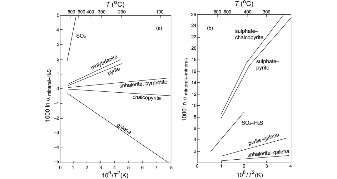
(a) Partitioning of 34S between minerals and H2S as a function of temperature. Mineral pairs with the greatest separation will be the most sensitive thermometers (data from Table 7.4a). (b) Partitioning of 34S between mineral pairs and SO2–H2S showing that the greatest fractionations are between sulphides and sulphates.
In contrast to the relatively small amount of sulphur isotope fractionation between sulphide mineral pairs, there is more extensive fractionation of δ34S between co-existing sulphide and sulphate phases. This can be seen in the relatively large fractionation factor between H2S and sulphate phases given in Table 7.4a and between sulphate and sulphide species listed in Table 7.4b. Rye (2005) reviewed the stable isotope geochemistry of sulphate–sulphide equilibria in igneous and fluid-related hydrothermal systems but found that there is frequently disequilibrium between coexisting sulphate and sulphide species. Rye (2005) recommends two different graphical techniques to establish equilibrium relationships. First, he uses a 1000 ln
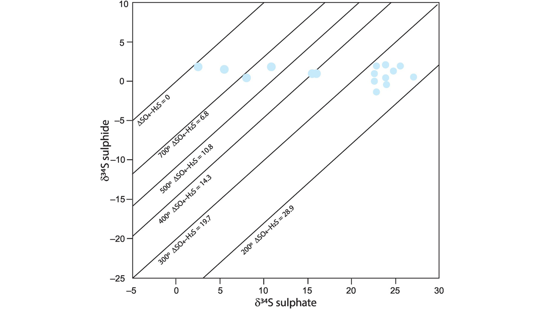
δ34Ssulphate versus δ34Ssulphide plot showing disequilibrium between coexisting sulphate and sulphide minerals in late Miocene magmatic and hydrothermal mineral deposits in the Julcani district of Peru.
(c) Sulphur isotope fractionation in sedimentary rocks. In marine sediments the sulphur cycle is driven primarily by the process of dissimilatory sulphate reduction (DSR), which is the reduction of seawater sulphate to sulphide by anaerobic microorganisms. This process can be thought of as a form of sulphate respiration. The metabolic pathway in these organisms converts sulphate into hydrogen sulphide. Much of the sulphide produced in this way is subsequently converted back into sulphate by a series of microbial and geochemical oxidation reactions, but some of the H2S combines with iron and organic matter and is buried in the sediment. Thus, the end product of this process is the formation of sedimentary pyrite. This part of the surface sulphur cycle is closely tied to the surface oxygen and carbon cycles (Rickard et al., 2017) and has implications for the evolution of the composition of the atmosphere, the oceans and the development of life (Figure 7.22).
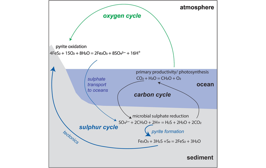
The relationship between the sulphur cycle and the surface carbon and oxygen cycles showing the principal chemical reactions.
There are two other significant biological processes which fractionate sulphur isotopes in the sedimentary environment. Assimilatory sulphate reduction is the means by which green plants, fungi and most bacteria reduce sulphate to sulphide. In this process, sulphide is produced for biosynthesis but there is no energy gain. In addition, there is the process of microbial disproportionation of sulphur (i.e., the simultaneous oxidation and reduction of sulphur) in which microbes disproportionate sulphur compounds with an intermediate oxidation state created during the re-oxidation of sedimentary sulphides, sulphites, thiosulphate and elemental sulphur.
The various redox reactions between the different sulphur species affect the isotopic composition of the resultant sulphides and sulphates. There are two main processes. First, there is kinetic fractionation, in which heavy isotopes have a reaction velocity which is slightly slower than light isotopes during the transformation of an oxidised to a reduced phase. In the conversion of sulphate to sulphide, the sulphide product is relatively enriched in the light isotope relative to the heavy isotope and so has a more negative value of δ34S. A second process is equilibrium fractionation, in which a heavy isotope (34S) is more stable when it is part of a strong bond, such as with oxygen in sulphate, and the lighter isotope (34S) is more stable when there is a weaker bond, such as with hydrogen in H2S (Jørgensen et al., 2019). The impact of these different microbial fractionations of sulphur isotopes was summarised by Shen and Buick (2004) as follows:
In dissimilatory sulphate reduction, sulphur isotope fractionation is relatively small; on average, the fractionation between δ34S of plants and their sulphate source is about −1.5‰.
In the case of assimilatory sulphate reduction, large fractionations have been recorded. In laboratory studies, fractionations of 70‰ are seen, although in natural populations the upper limit of fractionation is a depletion in 34S of 49‰.
During the re-oxidation of H2S produced by microbial sulphate reduction and the disproportionation of metastable intermediate compounds, there can be depletions in 34S of up to 70‰.
In addition to the microbial processes discussed, there are also abiogenic processes whereby sulphur isotopes are fractionated in the sedimentary environment. During the formation of evaporites the precipitation of sedimentary sulphate from seawater produces a relatively small δ34S enrichment of 1.65 ± 0.12‰ (Thode and Monster, 1965). In addition mineral deposits show evidence of sulphate reduction at temperatures above those favourable to sulphate-reducing bacteria (Trudinger et al., 1985). For example, in ocean-ridge hydrothermal systems sulphate reduction can be achieved by reaction with Fe2+-bearing minerals. It is likely that this is an equilibrium process in which the isotopic composition of sulphates in equilibrium with sulphides is isotopically heavier than that of the initial sulphate composition (Shen and Buick, 2004, and references therein).
7.3.4.3 Using Sulphur Isotopes to Identify Multiple Sources in Igneous Rocks and Hydrothermal Mineral Deposits
(a) Igneous rocks. The data in Figure 7.19 show that some suites of igneous rocks have a range of sulphur isotope ratios which cannot easily be explained simply by the relatively small fractionations which take place during igneous processes (Section 7.3.4.2). This is apparent in the data for arc basalts and granitoids and implies that these rock types are produced either from multiple sources with different sulphur isotope compositions or via a mixing process such as the crustal contamination of mantle-derived melts. An example of crustal contamination is given by Boztug and Arehart (2007) in their study of post-collisional granitoids from central Anatolia, Turkey. These granitoids have whole-rock sulphur isotope ratios of δ34S = 1.9–15.3‰ and show a positive correlation on a δ34S versus δ18O diagram, suggestive of mixing between mantle-derived melts (low δ34S and δ18O) and crustal melts (high δ34S and δ18O).
Massive sulphide ores associated with mafic and ultramafic rocks from the eastern part of the Central Asian Orogenic Belt in north-west China have δ34S values in the range 0.8–8.2‰ (Tang et al., 2012). These values are higher than those found in sulphides from mantle-derived melts and are interpreted as the result of contamination of mantle-derived melts with crust-derived sulphur with a positive δ34S. Gabbros and associated magmatic sulphides from the Hidaka metamorphic belt in Japan also preserve a record of crustal contamination of mafic magmas, in this case through magma mixing and the assimilation of a crust-derived tonalite which has a strongly negative δ34S signature. Tompkins et al. (2012) calculate that the δ34S ratios in the gabbros (δ34S = +6 to −7.5‰) can be modelled with an AFC process in which 10 wt.‰ tonalite (δ34S = −4.5 to −10.5‰) was mixed with the gabbro followed by about 14 wt.‰ fractional crystallization.
An example of mixing in a mantle source region is given by Dottin et al. (2020), who show that in the magmas of the Samoan mantle plume there is evidence of the mixing of two mantle sources. Samoan basalts display a positive correlation between δ34S and 87Sr/86Sr, implying a small but variable crustal component in the mantle source. They propose a model to explain the compositional variation in the melts in which there is mixing between an enriched component with slightly positive Δ33S and a positive δ34S, which they equate with the mantle source region HIMU, and a component with Δ33S = 0 and negative δ34S, which they regard as primordial mantle.
(b) Hydrothermal mineral deposits. Many hydrothermal mineral deposits form as a result of mixing of fluids derived from a number of different sources with different sulphur isotope compositions. Sulphur isotope studies therefore are an important tool in constraining their origin and mechanism of deposition. This is illustrated in Figure 7.23, which shows the wide range of δ34S compositions recorded in the sulphide and sulphate minerals from different types of hydrothermal mineral deposit. While this variability has been known and understood for some time, the recent application of in situ sulphur isotope measurements is opening up a much more nuanced approach to variations in the fluid chemistry (McDonald et al., 2018; Mukherjee et al., 2019).
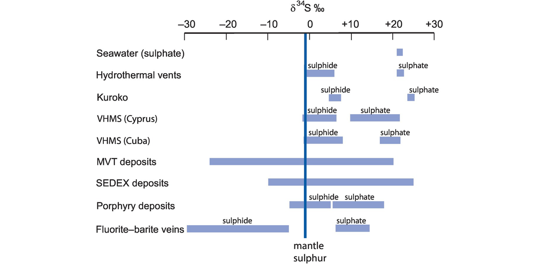
Sulphur isotope composition of sulphide and sulphate species in hydrothermal ore deposits relative to mantle sulphur.
Volcanic hosted massive sulphide deposits (VHMS), typified by modern hydrothermal vent systems forming at mid-ocean ridges and Kuroko-type deposits hosted in felsic calc-alkaline lavas, illustrate some of the end-member processes well, for at their simplest these systems represent the mixing of mantle-derived sulphur with δ34S ~ 0‰ and seawater sulphate with δ34S ~ 21‰. The δ34S values recorded in the different sulphide and sulphate phases from these deposits reflect this range of values and the associated processes of bacteriological sulphate reduction (Butler et al., 1998; Luders et al., 2001; Cazanas et al., 2008; Keith et al., 2016).
The δ34S values for most porphyry-type deposits are between −5.0 and +5.0‰, close to the mantle range (Han et al., 2018). In their study of the Donggebi porphyry Mo deposit in the Central Asian Orogenic Belt in China, Han et al. (2018) report a narrow range of δ34S values in molybdenite and associated sulphides of between 1.5 and 3.8‰. In this instance there are no marine sediments in the vicinity, but the fact that these values are elevated above typical mantle values suggest that they have interacted with a crustal source.
Sulphides from Mississippi Valley–type (MVT) ores show a large compositional range of between δ34S = −25 and +25‰ (Figure 7.23); individual deposits are also quite variable with ranges of δ34S up to 20–30‰. These large ranges are thought to be indicative of Rayleigh fractionation in partially closed systems where sulphate supply is the limiting factor. Deposits with negative values may result from the large fractionations produced by bacterial sulphate reduction in marine sediments. Those with positive values may reflect significant bacterial sulphate reduction in organic-rich settings or through thermochemical sulphate reduction in the subsurface (Shanks, 2013).
Sulphides in the Cretaceous fluorite–barite hydrothermal veins from the Freiberg ore district in Germany have a wide range of δ34S values between −5.5 and −30.9‰. Cogenetic barites have δ34S values between +6 and +14‰. This range of values is thought to indicate the mixing of two highly saline brines and the partial reduction of marine sulphate (Bauer et al., 2019).
7.3.4.4 Using Sulphur Isotopes to Understand the Evolution of the Earth’s Atmosphere
The discovery of mass-independent fractionation in the sulphur isotope system was unexpected and opened up an important means of understanding the nature of the atmosphere in the early Earth. Mass-independent sulphur isotope fractionation (Section 7.2.4) is thought to reflect photochemical processes in the upper atmosphere in which SO2 is reduced in ultraviolet radiation to elemental sulphur. The significant discovery, however, is that both the formation and the preservation of the mass-independent fractionation (MIF) signal require anoxic conditions. Experimental studies show that to create and preserve a MIF signal, oxygen concentrations have to be as low as 10−5 present atmospheric levels.
Early studies showed that both positive and negative Δ33S signals have been preserved. This is explained in terms of two different ‘channels’ from the atmosphere to the sediment where the signal is preserved. In the case of elemental sulphur created by the photolysis of volcanogenic SO2, this was transported to the Earth’s oceans in rain where it continued to exist either as elemental sulphur or as thiosulphate but ultimately was preserved in sediment as sulphide with a positive Δ33S signal. Alternatively, volcanogenic SO2 was converted into sulphite and sulphate in the atmosphere and transferred to the oceans as sulphate with a negative Δ33S signal. Some of this sulphate was preserved as sedimentary sulphate, while another component was converted into sedimentary sulphide with a negative Δ33S signal (Farquhar and Wing, 2003). Some of the sedimentary sulphide was subsequently returned to the mantle by means of subduction and recorded for posterity in tiny sulphide inclusions in diamonds (Farquhar et al., 2002).
Sulphur isotope data can be presented on a δ34S versus Δ33S diagram as a means of showing simultaneously the effects of mass-independent fractionation (Δ33S) relative to that of mass-dependent fractionation (δ34S). Ono (2017) has proposed that the Archaean reference array on this diagram has the slope Δ33S ~ 0.9 ∗ δ34S. An example of a δ34S versus Δ33S plot is given in Figure 7.24 and shows the composition of two groups of iron pyrites from the early Archaean of west Greenland. The data from sediments of the Isua greenstone belt have a clear MIF signal, whereas the samples from high-grade metamorphic rocks from Akilia Island show no MIF signal, perhaps indicating a non-sedimentary origin (Whitehouse et al., 2005).
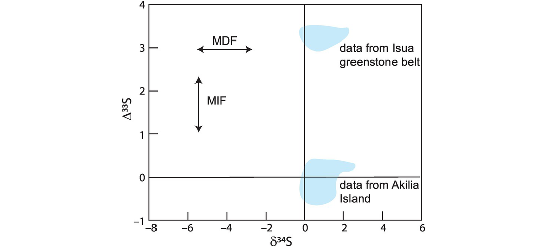
δ34S versus Δ33S diagram showing the composition of 3.7–3.8 Ga iron pyrites from west Greenland and the trends for mass-independent fractionation (MIF) and mass-dependent fractionation (MDF).
A plot of Δ33S over geological time shows that the MIF signal is present throughout the Archaean and is particularly well represented in the Neoarchaean, but then disappears completely from the geological record after 2.33 Ga (Figure 7.25). Given that the MIF signal is an indicator of an anoxygenic atmosphere, these data imply a significant increase in the oxygenation of the Earth’s atmosphere after 2.34 Ga, a finding which is consistent with other geological observations. This sharp increase in atmospheric oxygen is known as the Great Oxidation Event (GOE). It has been suggested that the plot of Δ33S over geological time might also imply some variability of oxygen levels throughout the Archaean, although it is important to note that the data from which this diagram is constructed are based upon a limited geographic distribution of samples (Ono, 2017).
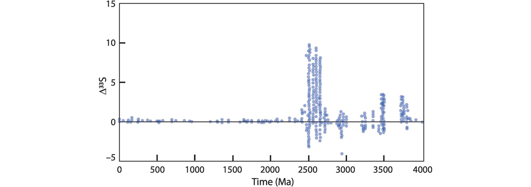
Plot of Δ33S versus time showing that the mass-independent fractionation signal is restricted to rocks older than 2.3 Ga, indicating the very low concentrations of oxygen in the Earth’s atmosphere before this time.
7.3.4.5 Using Sulphur Isotopes to Understand the Development of Early Life on Earth
As noted in Section 7.3.4.2, the low-temperature microbial reduction of sulphate to sulphide is accompanied by a large fractionation of sulphur isotopes such that pyrite produced by this process is strongly enriched in the light isotopes and has large negative δ34S values. This means, therefore, that the recognition of large negative δ34S values in the sedimentary record is a possible means of exploring the processes of microbial sulphate reduction in the geological past. This of course requires that primary biogenic signatures are preserved unmodified in the geological record. Fortuitously, sulphur is not remobilised in the sedimentary environment, for most sedimentary processes do not involve the transport of sulphur. Further, most biogenic sulphur is preserved as pyrite, and the additional isotopic fractionation associated with the conversion of microbial H2S to pyrite is low and is less than 1‰. This means that pyrite is potentially a robust ‘time capsule’ for the preservation of primary microbial signatures from the geological past, even to relatively high metamorphic grades (Shen and Buick, 2004; Rickard et al., 2017).
This is evident from studies of ancient sediments from as far back as the Archaean which in some instances preserve a wide range of sulphur isotope ratios which can be taken as a signal of biological activity in the form of microbial reduction of sulphate to sulphide. An example is the ~3.47 Ga sulphate-rich sediments of the North Pole area of north-western Australia described by Shen and Buick (2004). These samples contain sulphates with δ34S values between +3.2 and 5‰ and associated sulphides which show fractionations of between 7.4 and 21.1‰ relative to the sulphate. It is this fractionation which is interpreted as the signal of biological activity indicative of the process of dissimilatory sulphate reduction.
Samples from the 2.7 Ga Belingwe greenstone belt in Zimbabwe were investigated by Grassineau et al. (2005). They report a range of δ34S values from −21.1 to + 16.7‰ in sulphidic sediments. These values contrast with a probable mantle value of −0.5 ± 0.9‰ from associated volcanic rocks. These authors showed that even a single sample preserved domains which showed different degrees of sulphur isotope fractionation, which they suggested reflects a diverse range of coexisting microbial colonies.
Of course, when seeking to establish a biogenic signal from sulphur isotopes in ancient rocks, it is important to consider whether the signal could have been produced through non-biological activity. Reactions such as the re-oxidation of reduced sulphur species in repeated cycles and the disproportionation of intermediate sulphites into sulphide–sulphate mixtures can give rise to significant δ34S depletions. In addition, abiotic sulphur isotope fractionations can be the result of hydrothermal reactions. For this reason, establishing the validity of microbial activity in ancient sedimentary sulphide requires a full investigation of their setting using all the available geological and geochemical data.
7.3.5 Nitrogen Isotopes
Nitrogen occurs in nature as N2 gas, a highly volatile but inert component of the Earth’s atmosphere where it is present as 78‰ by volume. It also exists in multiple redox states as the reduced species NH4+ (ammonium), NH3 (ammonia) and in oxidised form as NO2− (nitrite) and NO3− (nitrate). To these ionic species human activity has added NOx (nitrogen oxides). Nitrogen is also an essential component of living organisms where it is present in amino acids, proteins and nucleic acids.
There are two naturally occurring isotopes of nitrogen: 14N (99.63‰) and 15N (0.37‰). Isotope ratios are measured as 15N/14N and expressed as δ15N‰ (Eq. 7.24) and measurements are made relative to the nitrogen isotopic composition of air (see Box 7.8). The variation in δ15N of the major terrestrial reservoirs is summarised in Figure 7.26.
Stable isotopes and abundances
Measured isotope ratios
Standards
AIR-N2, the nitrogen isotopic composition of air
Mantle value (depleted upper mantle)
Primordial mantle value
Bulk silicate Earth value
Variations in nature
See Figure 7.26.

Nitrogen isotope measurements are determined by conventional gas source ion-ratio mass spectrometry on the N2 molecule. Specialist sample preparation techniques are required when the sample size is very small which involve gas chromatography and dedicated combustion/reduction furnaces. In silicate rocks where concentrations are low, either static mass spectrometry or conventional ion-ratio mass spectrometry, using He as a carrier gas, allows sensitive measurements to be made (Cartigny and Marty, 2013). N-rich minerals such as nitrides and diamonds are amenable to analysis by ion-probe using a 133Cs+ primary beam.
A large fraction (~60‰) of the Earth’s nitrogen resides in the mantle (Bebout et al., 2013), and so it is important to consider the large-scale nitrogen cycle of the silicate Earth. At the Earth’s surface, organic nitrogen in sediments is converted into NH4+ and substitutes for K+ in clays and in detrital K-feldspar. In the crust the NH4+ is retained in residual mica during metamorphism and during partial melting nitrogen is retained as NH4+ in K-feldspar and as N2 in cordierite (Busigny and Bebout, 2013). Ultimately, nitrogen at the Earth’s surface is returned to the deep Earth by subduction; currently, there are two competing models for the mechanism whereby this takes place. It has been suggested that nitrogen is returned to the mantle via sediments in which the nitrogen is trapped in crustal minerals and bound in organic materials. More recently, Li et al. (2019) proposed that hydrothermally altered ocean crust, with positive δ15N values, is a more efficient mechanism for returning nitrogen to the Earth’s mantle.
At the Earth’s surface the significant part of the nitrogen cycle takes place in the ocean (Figure 7.27). Here biological nitrogen fixation (diazotrophy) is the process whereby atmospheric and dissolved N2 are converted to NH4 using the enzyme nitrogenase. The ammonium then either is oxidised to nitrogen and returned to the atmosphere or becomes fixed in organic matter and mineralised as kerogen. This then is either incorporated into sediments or oxidised to give marine nitrate. The marine nitrate may return nitrogen to the atmosphere, be converted into kerogen via marine organisms or be biologically assimilated and converted back into ammonium. All these exchanges are controlled by microbial activities which employ the following pathways:
Ammonification: this process includes both the fixation of nitrogen gas as ammonium and the reduction of nitrite (from nitrate) to ammonium
Nitrification: this involves the oxidation of ammonium to either nitrite or nitrate
Denitrification: the process whereby oxidised nitrogen species are reduced to N2 through one or more stages
Anammox (anaerobic ammonium oxidation): a process that simultaneously converts both ammonium and nitrite species to nitrogen (Stein and Klotz, 2016).
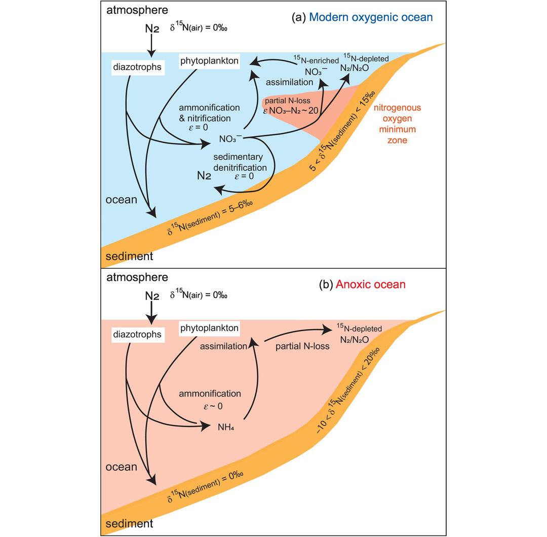
The nitrogen biogeochemical cycle in an oxygenic and an anoxic ocean; in each case the nitrogen cycle in the open ocean is shown on the left-hand side of the diagram and a zone of upwelling shown on the right-hand side of the diagram. (a) In a modern oxygenic ocean, diazotrophs and phytoplankton contribute both to organic matter in sediment and to the processes of ammonification and nitrification. In this scenario, ocean nitrate is partially denitrified and some is returned to organic matter through assimilation. In regions of upwelling through zones of low dissolved oxygen (nitrogenous oxygen minimum zone) more extreme isotopic fractionations are preserved in the sedimentary record and δ15N values increase. (b) In a fully anoxic ocean, nitrogen is supplied by N-fixation and by the generation of NH4 +. In this case there is no fractionation of nitrogen isotopes between the atmosphere and sediment. In zones of upwelling, the isotopic fractionation associated with NH4 + assimilation is expressed in the biomass, leading to both positive and negative fractionations and preserved in the sedimentary record. ε represents the fractionation between reactant and product ~ (δreactant – δproduct); where ε ~ 0‰ this indicates that the reaction is complete and there is no isotopic fractionation.
There are four main areas of contemporary geochemistry where the study of nitrogen isotopes is important:
In the modern Earth to aid understanding of biogeochemical cycles and as tracers of anthropogenic activity (Hastings et al., 2013)
In the deep Earth to improve our understanding of mantle processes from nitrogen isotopes in diamonds
In the early Earth for developing our understanding of ancient biogeochemical cycles, in understanding the redox state of the early oceans and in the understanding of the evolution of the Earth’s early atmosphere
In the search for life on other planets (Fogel and Steele, 2013).
7.3.5.1 The Distribution of Nitrogen Isotopes in Nature
The distribution of nitrogen isotopes in the Earth’s major reservoirs is summarised in Figure 7.26. It is thought that the nitrogen isotope composition of the Earth is close to that of chondritic meteorites, for when plotted on a D/H versus 15N/14N ratio diagram the Earth has a composition which lies between that of comets and the value for the solar wind (δ15N = −400‰), and is close to the values of carbonaceous chondrites (Marty, 2011; Cartigny and Marty, 2013). Further support for a chondritic model for nitrogen in the primordial Earth comes from the observation that the abundance of nitrogen on Earth is close to the chondritic value. On this basis, Jia and Kerrich (2015) proposed that the δ15N value for the bulk Earth can be calculated from a weighted mean of the values for enstatite chondrites (δ15N = −20‰ to −30‰) and carbonaceous chondrites (δ15N = +16‰ to +52‰) and calculated a bulk Earth value of δ15N = −7 ± 3‰, a value that overlaps with the δ15N value proposed for the modern mantle. In contrast to chondritic meteorites, iron meteorites have δ15N values in the range −100‰ to +155‰ (Murthy et al., 2019).
Nitrogen isotope measurements in fibrous diamonds and in vesicles in fresh mid-ocean ridge basalt glass suggest that the Earth’s depleted upper mantle has a value of −5 ± 2‰ and so is depleted in δ15N relative to the atmosphere (δ15N = 0). Some MORBs and OIB have higher values, indicating either that their source was contaminated with material from the Earth’s surface or that the δ15N values are elevated because of degassing. Nitrogen is only a minor component of volcanic gases but where measured in basaltic rocks tends to have values in the mantle range (de Moor et al., 2013).
Nitrogen substitutes for carbon in diamonds and so δ15N values in diamond can provide important information about mantle processes. Most diamonds have δ15N values in the range −12 to +5‰ with a mode of −5 ± 3‰, but some samples have values as low as δ15N = −40‰ and as high as +18‰ (Figure 7.26). It has been suggested that the wide range of positive δ15N values in diamonds might be evidence of the recycling of materials from the Earth’s surface into the deep mantle and that those diamonds with very low values of δ15N (~−40‰) could indicate the composition of the Earth’s primordial mantle (Cartigny and Marty, 2013). Rare micro-diamonds found in ophiolitic chromitites have δ15N values between −19 and +26‰ (Wu et al., 2019). A helpful way of representing the range of different diamond types is on a δ15N versus δ13C diagram, as illustrated in Figure 7.28.
Altered ocean crust has δ15N values which are higher than those recorded in the pristine crust and mantle. In detail, measured values are very variable and increase with increasing metamorphic grade: serpentinised meta-peridotite has δ15N = +4 to +15‰, altered and metamorphosed oceanic basalts δ15N = −11.6 to +8.3‰, ophiolitic metagabbros δ15N = +0.8 to +8.1‰ and eclogitic metabasalts δ15N = −1 to +8‰ (Busigny et al., 2018). Taken together these data imply that ocean crust which is returned to the mantle via subduction is likely to have a positive δ15N value.
In the Earth’s continental crust the dominant nitrogen species is NH4+ substituting for K+, Na+ and Ca2+ in illites, micas, feldspars, clinopyroxenes and amphiboles. In granitic rocks NH4+ is most abundant in biotite > muscovite > K-feldspar > plagioclase. An average δ15N value for the continental crust, based upon the composition of sedimentary and crystalline rocks, is δ15N ~ +6.0‰. This is consistent with the findings that most organic matter has δ15N = +3 to +7, that the devolatilisation of sediments during metamorphism leads to an enrichment in δ15N relative to the atmosphere and that granites have δ15N = +1 to +10‰ (Busigny et al., 2018).
Sedimentary rocks are the second most important reservoir of nitrogen at the Earth’s surface after the atmosphere. Nitrogen in sediments is preserved as organic nitrogen (in kerogen) and as fixed nitrogen in the form of NH4+ in phyllosilicates. Most sediments have δ15N values in the range −6 to +20‰ with an average value of δ15N = +7.2 ± 3.3‰. Marine sediments containing organic matter have δ15N values in the range +3 to +14‰ and are thought to reflect an aerobic oceanic cycle (Stüeken et al., 2016). The isotopic composition of marine nitrate is a product of the marine nitrogen cycle as illustrated in Figure 7.27 and δ15N values are between ~+1.0 and +15‰ with a mode of δ15N = +5 to +6‰ (Ader et al., 2016).
Given that the Earth’s continental crust (average δ 15N ~ +6.0‰) and atmosphere (δ15N = 0.0‰) were originally extracted from the mantle, it has been suggested from mass balance calculations that the mantle should have a positive δ15N value, rather than the observed δ15N = −5.0. Possible solutions to this paradox are that the δ15N value of the mantle has changed over geological time or that there are as yet unrecognised deep mantle reservoirs with lower δ15N than that of the depleted upper mantle (Cartigny and Marty, 2013).
7.3.5.2 Controls on the Fractionation of Nitrogen Isotopes
Fractionation between the different nitrogen species is not well known because the relevant fractionation factors are not yet sufficiently well determined. Some fractionation factors have been calculated theoretically (see Busigny and Bebout, 2013), although many carry a high degree of uncertainty. An empirical study by Petts et al. (2015) for diamond-bearing fluids has estimated a diamond–fluid N isotope fractionation factor (Δ15Ndiam–fluid; see Eq. 7.6) of −4.0 ± 1.2‰ at 1100°C. For more complex, carbon-poor fluids this value rises to ~−5.2‰. For fluids where NH3, N2 and NH4+ are the primary N species theoretical calculations based upon these observations yield Δ15Ndiam–fluid values at 1100°C of −1.4‰, −2.1‰ and −3.6‰, respectively (Petts et al., 2015).
Nitrogen has a similar solubility to that of Ar in the mantle and is thought to be incompatible. During partial melting the fractionation of nitrogen isotopes is thought to be small and at the per mil level (Cartigny and Marty, 2013). However, there is some evidence that nitrogen isotopes are fractionated during the degassing of basaltic melts. Cartigny and Ader (2003) calculated a shift from δ15N = −5.0‰ in the source to +3.0‰ after the degassing of OIB melts. Under reducing conditions nitrogen behaves as siderophile element in the silicate Earth and could therefore be present in the Earth’s core.
Within the modern oceanic nitrogen cycle there are a large number of different metabolic processes which give rise to a range of isotopic fractionations (Ader et al., 2016; Stüeken et al., 2016); however, given the wide range of redox states in the oceans and associated sediments, it is important to determine whether these fractionations take place under oxygenic or anoxic conditions (Figure 7.27). Denitrification and anammox are the dominant metabolic processes whereby marine nitrate is converted into atmospheric nitrogen, and these are the principal controls on the δ15N composition of the oceans and modern sediment. The net effect of these reactions leads to an enrichment of δ15N in the oceans of +5 to +7‰. This enrichment is then transmitted via marine organisms to sedimentary kerogen, which is then preserved in the sedimentary record with little further isotopic fractionation. Thus, under oxygenic conditions marine sediments approach the isotopic composition of NO3− in the overlying water column (Zerkle et al., 2017). Additional minor isotopic fractionation may occur by biological nitrogen fixation (diazotrophy) which produces a biomass with δ15N between about +1.0 and −1.0‰, the diagenetic remineralisation of organic-bound ammonium to dissolved NH4+ which renders the residual biomass isotopically heavier by 1.4–2.3‰ (Stüeken et al., 2016), and the release of ammonium from sediment (denitrification) which leads to nitrate which is isotopically lighter than the original biomass.
Most nitrogen in the geological cycle is preserved either in kerogen or as ammonium ions in potassic minerals, and with increased burial and metamorphism δ15N values in sedimentary rocks are enriched. Thomazo and Papineau (2013) suggested that values increase by 1–2‰ at greenschist facies, by 3–4‰ at amphibolite facies and up to 6–12‰ at upper amphibolite facies. Stüeken et al. (2017) show that for many metasediments the kerogen component is isotopically lighter than the silicate fraction and the bulk rock and that this difference becomes larger with increasing metamorphic grade, indicating an equilibrium isotopic separation between the kerogen-bound and silicate-bound nitrogen. These authors recommend that for samples metamorphosed up to greenschist facies and with >40‰ silicate-bound nitrogen, the primary isotopic composition of the biomass is best approximated by the bulk rock δ15N value, whereas for very kerogen-rich samples and rocks at higher metamorphic grades the δ15N values of the kerogen fraction are closer to that of the original biomass.
7.3.5.3 Using Nitrogen Isotopes as a Tracer in Geological and Biological Processes
Inspection of the δ15N values reported in Figure 7.26 shows that samples from the Earth’s surface environment have positive values and are higher than that of the Earth’s mantle. This is thought to reflect the influence of microbial processes. In contrast, some mantle-derived materials, notably, some diamonds, have highly negative δ15N values indicating that some mantle fluids and/or reservoirs are highly δ15N-depleted. These differences therefore provide a means of discriminating between a range of geological and biological processes in the Earth. For example, the variation in δ15N in sedimentary rocks can be used to track changes in the marine nitrogen biogeochemical cycle over geological time. As noted above, unaltered marine sediments that contain organic matter and have δ15N values in the range +3 to +14‰ are usually interpreted as reflecting an aerobic oceanic cycle. The details of specific microbial fractionations representing particular biogeochemical reactions have been summarised by Ader et al. (2016) and Stüeken et al. (2016).
In environmental geochemistry it has been shown that anthropogenic nitrogen in the form of NOx gases, and now recorded as nitrate, has a distinctive isotopic composition. Hastings et al. (2013) show that δ15Nnitrate values in Greenland ice cores have decreased from +11 to −1.0‰ since preindustrial times, indicating the effects of human activity in the use of fossil fuels and fertilizers. A particularly useful approach in the study of modern nitrates is to fingerprint them using the isotopes of both oxygen and nitrogen on a combined δ18O–δ15N plot (Hastings et al., 2013).
In the Earth’s mantle N isotope compositions can be combined with C isotope measurements and plotted together on a δ13C–δ15N diagram to identify different types of diamond (Figure 7.28; Wu et al., 2019). This diagram can also be used to understand the role of carbon- and nitrogen-bearing fluids in the mantle and to evaluate their role in the formation of diamond. In this way Smit et al. (2016) showed that mixed habit diamonds from Marange in Zimbabwe formed through the mixing of two different mantle fluids, one CH4-rich and the other CO2−/CO2-rich. The positive δ15N values for these fluids suggest their derivation from a metasedimentary source and therefore imply the dehydration of a subducting slab in their genesis.
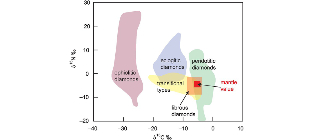
δ13C versus δ15N plot of diamond compositions showing the compositional range in diamond types relative to the modern (depleted) mantle value.
7.3.5.4 Using Nitrogen Isotopes to Understand Processes in the Early Earth
A number of authors have proposed that there is a secular trend in nitrogen isotope ratios for organic nitrogen as recorded in Archaean and Proterozoic sediments (Beaumont and Robert, 1999; Thomazo and Papineau, 2013). These authors found that kerogen in Archaean chert has average δ15N values of about 0‰, whereas in the early Proterozoic these values were about +5‰, a shift which is coincident with the Great Oxidation Event at ~2.34 Ga. However, unravelling the ancient nitrogen isotope record is not straightforward, for it is always necessary to assess whether or not the measured isotopic shift is the product of biogenic processes or the effect of later metamorphism (Thomazo and Papineau, 2013).
Before the GOE at ~2.34 Ga the lack of oxygen in the atmosphere would prohibit the oxygenation of the oceans and lead to a different set of metabolic pathways from the modern (Figure 2.27b). This is illustrated by Mettam et al. (2019), who show that 2.5–2.6 Ga shallow marine carbonates preserve evidence of an anaerobic nitrogen cycle dominated by N2 fixation and the assimilation and recycling of ammonium (δ15N = −3.3 to +3.2‰). In contrast, δ15N values from 2.31 Ga shales from the Rooihoogte and Timeball Hill formations in South Africa, formed after the GOE, provide evidence of an aerobic marine nitrogen cycle dominated by processes of nitrogen loss. In these rocks δ15N values in the upper part of the succession are 7.2 ± 1‰, close to modern marine values (Zerkle et al., 2017).
7.4 Non-traditional Stable Isotopes
Non-traditional stable isotopes are relative newcomers to the geochemical toolkit and have, for the most part, been in use for only the past two decades. Their advent has been made possible largely by the development of multi-collector inductively coupled plasma mass spectrometry (MC-ICP-MS). The development of this instrumentation has revolutionised the ability of geochemists to measure very small differences in isotope ratios for a large number of different isotope systems and provides a level of resolution sufficient to resolve the (usually) small differences found between natural samples.
When compared with the traditional stable isotopes (H, C, N, O, S) which have a relatively low atomic mass, the non-traditional stable isotopes include both heavy and light elements, many of which are trace elements and whose properties vary from volatile to refractory. Some occur in a number of different oxidation states and some have more than two isotopes and so offer potential insights through different types of mass fractionation (Teng et al., 2017b). Because of their geochemical versatility, the non-traditional stable isotopes offer potential insights into a wide range of geological, cosmochemical and bio-geochemical processes (Albarede et al., 2017).
A summary of the full range of non-traditional stable isotope systems currently being investigated by geochemists is shown on the periodic table in Figure 7.29. Here the elements are divided into those whose stable isotope geochemistry is not currently so well known – the ‘emerging non-traditional isotope systems‘ as defined by Teng et al. (2017b) – and those stable isotope systems which are relatively well studied. Of the latter, five are selected here for more detailed discussion: Li, Mg, Si, Cr and Fe.
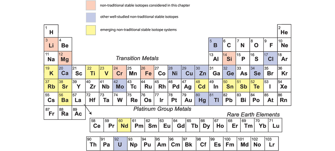
Periodic table of the elements showing the non-traditional isotope systems currently being investigated in geochemistry. The elements are identified either as having isotope systems which are relatively well-studied (blue) or as having stable isotope systems which are still emerging (yellow) (after Teng et al., 2017b). The isotope systems discussed in this section are highlighted in pink.
Some of the non-traditional stable isotope systems show only small amounts of fractionation and until the advent of precise MC-ICP-MS measurements rendered them out of reach of isotopic analysis. This is in part linked to the small relative mass differences that occur between the stable isotopes of the heavier elements. Figure 7.30 illustrates the natural terrestrial variation between isotopes in the different non-traditional isotope systems discussed here and their relative mass differences.
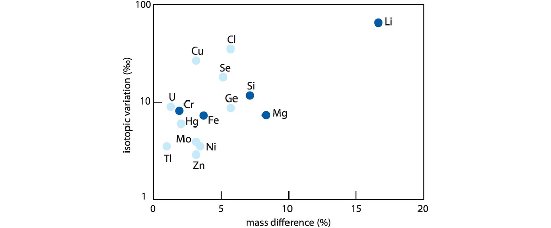
Plot of the non-traditional stable isotopes used in this section showing the extent of their natural isotopic variation (‰, log scale) versus the relative mass difference between the isotopes used in the calculation of the isotopic ratio (%). The isotopes shaded dark blue are those discussed in detail in this chapter.
In addition to solution MC-ICP-MS important advances have also been made in the application of in situ techniques. These involve the use of laser ablation MC-ICPMS and MC-SIMS (ion microprobe) technologies (Chaussidon et al., 2017). The SIMS approach offers high spatial resolution (10–20 μm), high sensitivity and low background interference. The sensitivity of the LA-MC-ICPMS technique is in part dependent on the choice of laser and the ablation efficiency. Other analytical considerations are that the very small volume of material sputtered or ablated may limit the possible precision; the ion yield of samples may vary as a function of the composition of the sample matrix; and there can be isotopic fractionations within the instrument itself (see the review by Chaussidon et al., 2017).
For a fuller discussion of non-traditional stable isotopes the reader should consult the review volumes edited by Johnson et al. (2004), the updated version edited by Teng et al. (2017a) and the recent edition of Hoefs (2018). Titles specific to individual isotopes include the volume by Tomascak et al. (2016) on Li isotopes and Johnson et al. (2020) on Fe isotopes.
7.4.1 Lithium Isotopes
Lithium occurs most commonly as a trace element, and in octahedral coordination the Li+ ion has a similar size to that of Mg2+. For this reason Li tends to substitute for Mg in silicate minerals. There are two isotopes, 6Li and 7Li, and the relatively large mass difference means that there can be significant mass fractionation in excess of 50‰ (Figure 7.30). Li isotopes are measured as 7Li/6Li and expressed as δ7Li (Eq. 7.25) relative to the synthetic standard IRMM-016. The isotope systematics of Li are summarised in Box 7.9. Li is present only as monovalent Li+, and so its isotopic composition is not influenced by redox states. The original pioneering work in Li isotope geochemistry was carried by L.-H. Chan of Louisiana State University using thermal ionisation mass spectrometry (Chan, 1987), although this method has now been superseded by MC-ICP-MS. A fuller discussion of the application of Li isotopes is given in the recent book by Tomascak et al. (2016) and in the review article by Penniston-Dorland et al. (2017).
In low-temperature environments at the Earth’s surface there are large Li isotope fractionations between minerals and an aqueous fluid phase. This means that materials from the Earth surface, such as hydrothermally altered oceanic basalts and the products of continental weathering, have distinctive isotopic compositions which have the potential to be traced through the processes of recycling back into the Earth’s mantle. There appear to be no biological controls on the fractionation of Li isotopes, and so δ7Li values in carbonate rocks offer the potential for providing a record of the Li isotopic composition of seawater. At high temperatures the differential diffusivity of the two Li isotopes is important in diffusion studies and offers the potential for studying rates of cooling in igneous rocks (Penniston-Dorland et al., 2017).
Stable isotopes and abundances
Measured isotope ratios
Standards
Originally, L-SVEC, a Li-carbonate (NIST standard reference material 8545)
Now replaced by IRMM-016 (Penniston-Dorland et al., 2017)
Mantle value
Bulk silicate Earth value
Variations in nature See Figure 7.31.
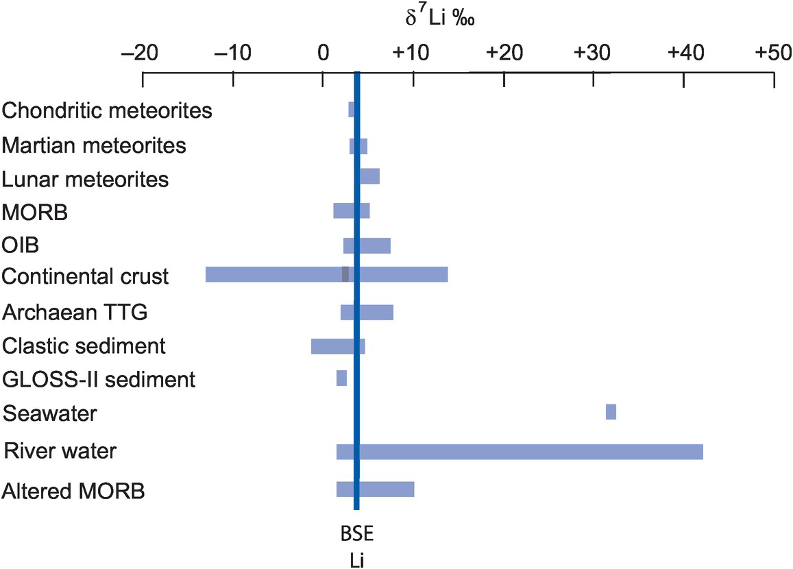
Variation in δ7Li in extra-terrestrial and terrestrial reservoirs relative to the bulk silicate Earth (BSE).
7.4.1.1 The Distribution of Lithium Isotopes in Nature
The distribution of Li isotopes in the common terrestrial and extra-terrestrial reservoirs is summarised in Figure 7.31. Chondritic δ7Li values are between +3 and +4‰, although in situ measurements of individual chondrules show a much greater range of values, indicating significant heterogeneity both within and between samples. In other extra-terrestrial bodies Martian meteorites have δ7Li values in the range +2.1 to +6.2‰, with an average of +4.2 ± 0.9‰, thought to represent the bulk silicate composition of Mars. Lunar meteorites have δ7Li values in the range +3.5 to +6.6‰ (Penniston-Dorland et al., 2017).
Interpreting δ7Li values from mantle peridotites is complicated because of the effects of high-temperature diffusion in mantle minerals and later metasomatic overprinting. Bulk-rock peridotite δ7Li values range from −9.7 to +9.6‰, but data from carefully selected unmetasomatised, fertile peridotites which are isotopically equilibrated show a much narrower range of δ7Li values between +3.5 to +4.0‰, and this is taken to be the bulk silicate Earth value. δ7Li measurements in unaltered MORB lie between +1.6 and +5.6‰ (average δ7Li = 3.4 ± 0.7‰); OIB samples have a similar range δ7Li = +2.4 to +7.9‰ (average 3.8‰) as do arc basalts (average δ7Li = 3.6 ± 1.2‰) (Penniston-Dorland et al., 2017, and references therein). The similarity in Li isotope composition between MORB and OIB suggests that the upper and lower mantle have a similar average Li isotope composition.
The average composition of the upper continental crust, as estimated from loess, is δ7Li = 0.6 ± 0.6‰ (Sauzeat et al., 2015). The average δ7Li for the middle continental crust is +4.0 ± 1.4‰, whereas granulites from the lower continental crust are more heterogenous; equilibrated samples are in the range δ7Li = −14 to +14.4‰, with an average of δ7Li = 2.5‰. Using the relative crustal proportions of Rudnick and Gao (2014) these values suggest that an average bulk crust (17 ppm Li) has a δ7Li value of ~2.3‰. This is close to the value for average global oceanic subducted sediment (GLOSS-II), which has a value of δ7Li = 2.4 ± 0.02‰. Archaean tonalite–trondhjemite–granodiorites (TTGs) have values in the range 2.5–7.5‰ with a mean value of 4.3‰ (Liu and Rudnick, 2011).
The Li isotopic composition of seawater is δ7Li = +31 ± 0.05‰, isotopically much heavier than the crust and the mantle. This value is the result of inputs from the dissolve load in rivers (average δ7Li = +23‰, range +1.0 to +44.0‰), groundwater (δ7Li = +15‰) and hydrothermal vent fluids (δ7Li = +7.2 to +8.9‰; Foustoukos et al., 2004) and the loss of δ7Li to clays during the hydrothermal alteration of ocean basalts. MORB altered as a result of interaction with seawater becomes isotopically heavier and has a δ7Li value of 5.6 ± 4.5‰, whereas there is some evidence that mantle peridotites altered to serpentinite become isotopically lighter (Hansen et al., 2017; Penniston-Dorland et al., 2017, and references therein).
In a review of the Li isotope composition of marine sediments from a wide range of tectonic settings, Chan et al. (2006) show that the bulk δ7Li of global sediments varies between −4.3 and +14.5‰ and that there are large differences between different types of sediment. For example, detrital sediments such as turbidites and clays are in the range −1.5 to +5‰ with clays isotopically lighter than sands because of isotopic fractionation during continental weathering. Volcanogenic marine sediments may be either heavier or lighter than the mantle value depending on the extent to which they have interacted with seawater. Biogenic sediments – carbonates and silica-rich sediments – tend to recrystallise during diagenesis, leading to isotopically heavier compositions (+6 to +14.5‰).
7.4.1.2 Controls on the Fractionation of Lithium Isotopes
In ferromagnesian minerals, lithium commonly substitutes for Fe–Mg in octahedrally coordinated sites, although in aqueous fluids it is thought to reside mostly in tetrahedrally coordinated sites. This gives rise to the preferential equilibrium partitioning of 7Li into aqueous fluids relative to ferromagnesian minerals, so that aqueous fluids in contact with mafic rocks will be enriched in δ7Li. Experimental studies show that at high temperatures these mineral–fluid fractionations are relatively small but at lower temperature the fractionations are large. Thus, low-temperature mineral reactions such as the formation of clays can result in large isotopic fractionations. Studies show that 6Li is preferentially incorporated into clay, whereas the host fluid in equilibrium with the clay becomes enriched in 7Li. In a similar way the carbonate minerals calcite and aragonite show significant isotopic fractionation relative to aqueous fluids enriching the equilibrium fluid in 7Li. Experimentally determined mineral/rock–fluid fractionation factors for a range of geological materials are given in the review by Penniston-Dorland et al. (2017).
At high temperatures kinetic fractionations are important in the Li isotope system as a result of the more rapid diffusion of 6Li relative to 7Li. Large fractionations have been recorded in magmatic and metamorphic rocks (up to 20‰) and over tens of metres, although the evidence of fractionation will survive only in systems that cool rapidly (Penniston-Dorland et al., 2017, and references therein).
7.4.1.3 Using Lithium Isotopes as a Tracer in Geological Processes
Li isotopes can be used to understand igneous processes, as well as to investigate weathering processes.
(a) Li isotopes in understanding igneous processes. As has been noted for other stable isotope systems, the equilibrium fractionation of isotopes on the basis of their mass differences is inversely proportional to temperature, so that at high temperatures there is minimal fractionation. This principle is true for lithium isotopes and implies that for unaltered mafic rocks their isotopic composition is indicative of the composition of their mantle source. Lithium behaves as a moderately incompatible element during partial melting, and there is very little Li isotope fractionation during this process. Further, there is no strong evidence to indicate that significant mineral–silicate melt fractionation takes place during magmatic differentiation in mafic rocks. Exceptions may be related to fluid processes such as magmatic degassing (Neukampf et al., 2019) and the exsolution of a supercritical fluid (Li et al., 2018). However, the moderately incompatible nature of Li means that it is concentrated in the crust relative to the mantle and so can be used to detect crustal contamination in mafic melts. This was demonstrated by Genske et al. (2014), who found a wide range in δ7Li values in OIB from the Azores (+3.5 to +8.5‰) and showed using AFC modelling that their mantle source had been contaminated with hydrothermally altered oceanic crust. At high temperatures the rapid diffusivity of Li in silicate minerals coupled with significant kinetic Li isotope fractionation during diffusion means that the Li isotope system has great potential as a geo-speedometer with which rates of cooling in igneous rocks might be investigated (Richter et al., 2017; Marschall and Tang, 2020).
Given the well-established Li isotope partitioning between silicate minerals and aqueous fluids it was expected that fluids released from a subducting slab containing hydrothermally altered oceanic crust would be enriched in δ7Li and that this signature would be imparted to the overlying mantle wedge and the resultant arc lavas. However, no obvious δ7Li imprint on arc lavas has been found, although there is some evidence for the incorporation of subducted sediment in arc lavas. Tang et al. (2014) found that the lavas in Martinique in the Lesser Antilles are isotopically lighter than MORB with δ7Li values = +1.8 ± 1.3‰ as are the associated sea-floor sediments (δ7Li = −4.4 to −0.5‰) leading them to propose that the composition of the lavas reflects a mantle source that had incorporated isotopically light subducted sediment.
In a similar way it was expected that since the Li isotope signature of hydrothermally altered crust (average δ7Li = 5.6 ± 4.5‰) is sufficiently different from that of MORB (average δ7Li = 3.4 ± 0.7‰), it would be possible to track subducted altered oceanic crust in the sources of MORB and OIB. In support of this view, Chan and Frey (2003) reported δ7Li from OIB from the Hawaiian plume of between 2.5 and 5.7‰ and proposed that this variability might reflect the minor influence of recycled oceanic crust. Similarly, Elliott et al. (2006) reported δ7Li values for fresh MORB glasses from the East Pacific Rise in the range 3.1–5.2‰, which they interpreted as coming from a mantle source which had been enriched by the incorporation of recycled mantle wedge material. However, more recently it has become clear that Li isotope data of this type must be treated with caution because of the diffusive fractionation of Li at high temperatures (Marschall and Tang, 2020).
(b) Li isotopes in understanding the processes of continental weathering. Empirical studies have shown that during the weathering of silicate rocks Li is soluble and that 6Li partitions into the products of chemical weathering such as clays, whereas 7Li partitions into the associated water. In detail, weathering is a two-step process. Initially, minerals are dissolved and then secondary phases are precipitated. Typically, Li isotopes are not fractionated during the dissolution stage but are strongly fractionated during the formation of secondary weathering products. This means that the terrestrial weathering products of the continental crust are depleted in δ7Li but rivers are enriched in δ7Li. This has been demonstrated in the detailed examination of weathering profiles which show that the degree of Li isotope fractionation is controlled by the type of secondary minerals formed which in turn is related to the intensity of the weathering and climatic conditions during weathering (Teng et al., 2010).
Given that Li isotopes are not fractionated by biological processes, riverine Li isotopes serve as an important record of weathering process via their dissolved and suspended loads. While rivers are complex dynamic systems and may display mixing of water from different sources (Henchiri et al., 2016), empirical studies indicate three main characteristics. First, the Li isotope signature of the dissolved load of a river reflects the degree of chemical weathering in the region. Second, the difference in δ7Li between the dissolved and the suspended load can be related to the intensity of the weathering, with the greater δ7Li fractionation correlated with the greater weathering intensity (Pogge von Strandmann et al., 2006). Third, a recent study of weathering in the permafrost of eastern Siberia showed that climate also exercises a weak control on river Li isotope chemistry (Murphy et al., 2019).
Using these insights, Liu and Rudnick (2011) used Li isotopes to argue that chemical weathering has played a significant role in the evolution of the composition of the continental crust over geological time and attempted to constrain the mass of continental crust lost over time via this process. They argued that since the Li isotope composition of the continental crust is lower than that of the mantle-derived materials from which it was built, the missing δ7Li must have been returned to the mantle as a consequence of weathering and dissolution. Using a mass balance model for the Li isotope composition of the present-day bulk continental crust, they calculated that between 15 and 70‰ (mean value 45‰) of the original juvenile crust has been lost over geological time through weathering and dissolution.
Li is well mixed in seawater and so organisms that have grown in equilibrium with seawater will preserve a record of its former composition. This has been investigated using carbonate foraminifera. Misra and Froelich (2012) show that since the Eocene–Palaeocene (60 Ma) planktonic foraminifera have increased in their δ7Li from ~22‰ to the present-day value of 31‰. They argue this change in seawater chemistry represents a pattern of chemical weathering of continental rocks during the Eocene which is different from that in the modern, resulting in a lower riverine δ7Li 60 Ma ago.
7.4.2 Magnesium Isotopes
Magnesium is found in silicate rocks and the oceans and is an essential element in the biosphere. It is present as a major component in ferromagnesian minerals, carbonates, sulphates and clay minerals in igneous, metamorphic and sedimentary rocks. There are three isotopes of magnesium – 24Mg, 25Mg and 26Mg – and isotope ratios are measured as 26Mg/24Mg, expressed as δ26Mg‰ (Eq. 7.26) relative to a synthetic standard (Box 7.10). The range of fractionation found in most terrestrial materials is between ~−6 and +2‰ (Figure 7.32); this range is small compared with other stable isotope systems (Figure 7.30).
The measurement of Mg isotopes requires very high precision and must be carried out with great care, for analytical artefacts can arise through instrumental mass fractionation during analysis and from matrix effects. A detailed discussion of Mg isotope analysis using both ion-probe and ICP-MS technologies is given by Chaussidon et al. (2017) and Fukuda et al. (2020). A comprehensive review of the geochemistry of magnesium isotopes is given by Teng (2017) and a summary of the systematics is given in Box 7.10.
Stable isotopes and abundances
Measured isotope ratios
Standards
Dead Sea Magnesium (DSM3)
Cambridge-1 (this standard is 2.623 ± 0.030‰ lower than DSM3 (Teng, 2017), as solutions in nitric acid
Additional reference values for a range of silicate rocks and carbonates are given in Teng (2017).
Chondritic value
Mantle and bulk Earth value
Variations in nature
See Figure 7.32.
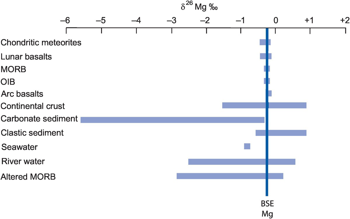
Variation in δ26Mg in extra-terrestrial and terrestrial reservoirs relative to the value in the bulk silicate Earth (BSE)
7.4.2.1 The Distribution of Magnesium Isotopes in Nature
Even though there is a relatively large mass difference between the isotopes 24Mg and 26Mg (~8‰), the degree of magnesium isotope fractionation found in both terrestrial and extra-terrestrial reservoirs is small (Figure 7.32). Chondritic meteorites of all classes have δ26Mg values in the range −0.43 to −0.15‰, with an average δ26Mg = −0.27 ± 0.12‰. Lunar values, derived from lunar basalts, are similar, with an average δ26Mg = −0.26 ± 0.16‰. A small difference in δ26Mg between high-Ti and low-Ti lunar basalts could suggest some heterogeneity in the source, perhaps indicating some fractionation during the early differentiation of the lunar magma ocean. Bulk silicate Mars is δ26Mg = −0.271 ± 0.040‰ (Magna et al., 2017). Unmodified mantle peridotite xenoliths also have a similar average value of δ26Mg = −0.25 ± 0.04‰. Metasomatized samples, that is, those whose composition has been modified by the migration of mafic melts, show a wider range of values. Given the highly magnesian nature of the Earth’s mantle, the mantle peridotite value is taken to be equivalent to that of the bulk silicate Earth (Figure 7.32). Taken together, the overall similarity in Mg isotope compositions of the Earth, the Moon, Mars and chondrites indicates that there was substantial Mg isotopic homogeneity in the early solar system, reflecting extensive early disc mixing (Teng, 2017).
Magnesium isotope measurements are similar in both MORB and OIB, with δ26Mg between −0.31 and −0.19‰ in MORB (average = −0.25 ± 0.06‰) and δ26Mg between −0.35 and −0.18‰ in OIB (average = −0.26 ± 0.07‰), indicating that the mantle is homogeneous and that there are no differences in δ26Mg between upper and lower mantle sources. Altered ocean crust is isotopically much more heterogeneous, with δ26Mg values between −2.76 and +0.21‰ and hydrothermally altered peridotites vary in δ26Mg between −0.25 and −0.02‰. In both instances these changes are largely the result of the formation of secondary clay-rich minerals formed during the hydrothermal weathering (Teng, 2017, and references therein). Arc lavas from the Lesser Antilles have δ26Mg values between −0.25 and −0.10‰, slightly heavier than in the mantle and MORB, suggesting that the sub-arc mantle source has been modified by the release of fluids enriched in δ26Mg from hydrothermally altered ocean crust in the subducting slab (Teng et al., 2016).
Magnesium isotope ratios in the continental crust are as follows: upper continental crust δ26Mg = −1.64 to +0.92‰, the middle crust δ26Mg = −0.40 to +0.12‰ and the lower crust δ26Mg = 0.76 to −0.24‰. The bulk continental crust average for δ26Mg = −0.24‰, a value that is very close to that of the mantle, reflecting the very small Mg isotope fractionations that take place during high-temperature igneous and metamorphic processes.
The magnesium isotope composition of seawater is δ26Mg = −0.83 ± 0.09‰; rivers are more variable in composition, with values between δ26Mg = −2.5 and +0.64‰. Rainwater and groundwater have slightly smaller ranges than that of river water, with δ26Mg = −1.59 to −0.51‰ (average −0.85 ± 0.58‰) and δ26Mg = −1.7 to +0.23‰ (average −1.23 ± 0.89‰), respectively.
Carbonate-rich sediments show the largest isotopic variation in Mg isotopes of all natural materials and have δ26Mg between −5.57 and −0.38‰. Relative to aqueous solutions abiogenic carbonates preserve fractionations of up to ~4.8‰. Dolomitic samples are at the heavy end of this range, whereas calcitic samples are lighter, indicating some mineralogical control on Mg isotope fractionation. In biogenic carbonates large fractionations of δ26Mg > 4.5‰ have been observed, giving rise to carbonates which are isotopically lighter than seawater. Marine sediments adjacent to subduction zones have δ26Mg values in the range −3.65 to +0.52‰ with calcareous oozes contributing to the lighter values and clastic materials the heavier values. Clastic sediments have δ26Mg between −0.57 and +0.92‰ (Teng 2017).
7.4.2.2 Controls on the Fractionation of Magnesium Isotopes
The data in Figure 7.32 show that the most extreme Mg isotope fractionations take place at low temperatures at the Earth’s surface and that they are particularly pronounced in carbonate rocks. The similarities in δ26Mg between average MORB, average OIB and average mantle peridotite suggest that there is no measurable equilibrium fractionation of magnesium isotopes during the process of the partial melting of the mantle. Further, Teng et al. (2007) showed that magnesium isotopic compositions do not change significantly during magmatic differentiation. They found that differentiated basalts and associated olivine-rich cumulates from Kīlauea Iki lava lake in Hawai‘i have Mg isotope compositions similar to that of the parental magma. In metamorphic rocks Teng (2017) showed that in silicate rocks there is no measurable Mg isotopic fractionation during metamorphism. This means that even at high grades of metamorphism, silicate metamorphic rocks preserve the isotopic composition of their protolith, although this is not the case in marbles where there is evidence of Mg isotopic exchange between carbonate and silicate minerals.
Evidence of high-temperature kinetic isotopic fractionation of Mg isotopes has been observed in some olivine phenocrysts in mafic melts. Coupled Mg elemental and isotopic zoning is indicative of Mg diffusion, and fractionations of up to 0.45‰ have been reported. There is also evidence for inter-mineral Mg isotope fractionation during the sub-solidus disequilibrium exchange of Mg isotopes between olivine and chromite in disseminated mantle chromitites (Xiao et al., 2016).
At low temperatures fractionations are more pronounced, but not particularly well understood. Experimental studies on the precipitation of carbonate minerals from aqueous solutions indicate that Δ26Mgaragonite–fluid is between −1.1 at 25°C and −0.8 at 55°C, Δ26Mgdolomite–fluid between −0.93 at 130°C and −0.65 at 220°C, Δ26Mgmagnesite–fluid between −1.2 at 150°C and −0.88 at 200°C and Δ26Mgcalcite–fluid is ~−2.1 at 25°C. Combining theoretical with experimental studies indicates an enrichment in 26Mg in carbonates in the order aragonite > dolomite > magnesite > calcite (Teng, 2017, and references therein).
The alteration of oceanic basalt in marine hydrothermal systems has been studied experimentally by Voigt et al. (2020). These authors show that isotopically heavy Mg is preferentially incorporated into basalt as the secondary clay mineral smectite, leaving a residual fluid enriched in light Mg isotopes. They calculate a smectite–liquid fractionation factor of 0.42‰ at 250°C.
7.4.2.3 Using Magnesium Isotopes as a Tracer in Geological and Biological Processes
It was shown above that there is minimal fractionation between Mg isotopes at high temperatures. This means that in igneous rocks the Mg isotope composition of basalts can be used to characterise their mantle source, and in granites Mg isotopes can be used to track the Mg isotope composition of the protolith. Similarly, the lack of fractionation in metamorphic rocks means that in silicate rocks, even at high metamorphic grades, the Mg isotopic composition will mirror that of the protolith.
In contrast, in the low-temperature environments of the Earth’s surface Mg isotopes are more extensively fractionated. A number of studies have shown that during continental weathering Mg isotopes are more variable in the dissolved and the suspended loads of the associated rivers than in the parent bedrock, indicating that isotopic fractionation takes place during the weathering process. This is evident from the study of weathering profiles. In the case of granite weathering, the fractionation is controlled principally by the formation of illite (Brewer et al., 2018), although in detail the magnitude of the Mg isotope fractionation during continental weathering depends upon the precise weathering processes involved and the clay minerals that are formed (Teng, 2017).
Magnesium is also an essential element in the biosphere, and there is evidence from laboratory experiments and in natural samples that Mg isotopes are fractionated during photosynthesis, although the extent of the fractionation depends upon both the plant species and the environmental conditions. In natural samples plants and trees prefer heavy Mg isotopes relative to their substrate, giving rise to Mg isotope fractionation during Mg transport (Teng, 2017).
The extensive isotopic fractionation of Mg isotopes in the low-temperature environments of the Earth provides an important potential tool for recognising the recycling of surficial materials into the Earth’s mantle by means of subduction and provides a distinctive Mg isotope signal in the sub-arc mantle and in arc lavas. However, apart from recognising recycled carbonated oceanic crust (Chen et al., 2018), this geochemical signal is proving elusive. Hu et al. (2020) found no difference between the Mg isotope composition of xenoliths from the mantle wedge of the Kamchatka Arc and that of ambient mantle, although they did find some variability in the Mg isotope composition of the arc lavas, which might be related to the recycling of Mg isotopes from subducted oceanic crust.
7.4.3 Silicon Isotopes
Silicon is abundant in the Earth and occurs mostly in the tetravalent oxidation state bonded with oxygen in silicate minerals or silica. In solution it is found as orthosilicic acid (H4SiO4 or Si(OH)4) and it occurs as Si0 when alloyed with metals in planetary cores. Silicon is also an essential structural component in plants and is found in some plankton and siliceous sponges. Silicon has three naturally occurring stable isotopes: 28Si, 29Si and 30Si. The isotope ratio measured is 30Si/28Si, expressed as δ30Si‰ (Eq. 7.27) relative to the NBS28 standard. Mass-dependent silicon isotope fractionation on the Earth has a range of about 12‰; the isotope systematics for stable silicon isotopes are summarised in Box 7.11. Comprehensive reviews of silicon isotope geochemistry are given by Zambardi et al. (2013), Savage et al. (2014), Poitrasson (2017) and Ledevin (2019).
Stable isotopes and abundances
Measured isotope ratios
Standards
RM 8546, for which δ30Si = 0.0‰, distributed by National Institute of Standards and Technology, NIST; also known as NBS28, sand quartz.
Formerly: Caltech Rose Quartz Standard (RQS)
Chondritic value
Bulk silicate Earth value
Variations in nature
See Figure 7.33.

Silicon isotopes are analysed by high-resolution MC-ICP-MS with a long-term reproducibility of ± 0.08‰. Sample preparation includes bulk sample alkali fusion and element purification using ion-exchange chromatography. A finer spatial resolution can be obtained using the microbeam techniques SIMS and LA-MC-ICP-MS, although these methods offer slightly lower analytical precision than high-resolution MC-ICP-MS. A full discussion of analytical approaches is given in Savage et al. (2014) and Poitrasson (2017).
The largest silicon isotope fractionations are found in the Earth’s surface environment (Figure 7.33), and these offer scope for deciphering past terrestrial environments and processes in the oceans. There is little silicon isotope fractionation during metamorphism, and so ancient sediments may record their primary silicon isotope compositions. In high-temperature igneous geochemistry there are important applications of silicon isotope geochemistry in the understanding of crust–mantle interactions during continent formation in the early Earth and in cosmology in the study of the processes of planetary formation.
7.4.3.1 The Distribution of Silicon Isotopes in Nature
Silicon isotope measurements in chondritic meteorites are in the range δ30Si = −0.41 to −0.64‰. δ30Si values for carbonaceous chondrites (−0.41 to −0.45‰) and ordinary chondrites (−0.46 to −0.49‰) are within error of each other and together have a mean value of −0.46 ± 0.02‰. Enstatite chondrites are isotopically lighter and have δ30Si values between −0.59 and −0.64‰. In contrast to the narrow range of values within chondritic meteorites, rare pre-solar SiC grains found included in chondrites show extensive fractionation with a range of 2000‰, which is thought to reflect nucleosynthetic processes in the universe prior to the formation of the Sun. Basaltic samples from the Moon yield a bulk silicate moon δ30Si value of −0.27 ± 0.02‰ and Martian meteorites of igneous origin have δ30Si = −0.56 to −0.33‰, with a bulk silicate Mars value of −0.49 ± 0.03‰, similar to the chondritic value (Zambardi et al., 2013).
The δ30Si value of the bulk silicate Earth based upon samples of mantle peridotite and basalt is −0.29 ± 0.07‰ (Savage et al., 2014; Deng et al., 2019). Averages of the samples used to calculate this value are as follows: ultramafic rocks δ30Si = −0.30 ± 0.09‰, MORB δ30Si = −0.27 ± 0.06‰, OIB δ30Si = −0.31 ± 0.04‰, Archaean komatiite δ30Si = −0.29 ± 0.02‰, and island arc basalts δ30Si = −0.28 ± 0.04‰. Felsic rocks have heavier δ30Si values and rhyolites from Hekla volcano in Iceland have values of ~−0.15‰. Savage et al. (2014) proposed an algorithm for igneous rocks in which δ30Si is linked to the SiO2 content of the melt, such that for mantle-derived equilibrium melts
Granites have δ30Si values in the range −0.40 to −0.11‰ (average −0.23 ± 0.15‰), lighter than expected from the igneous range given above in Eq. 7.29. Deng et al. (2019) showed that the variability within the range of granite compositions may be related to the protolith composition, for there is a difference between average δ30Si values for I- and A-type granites (−0.18 ± 0.02‰) and for S-type granites (−0.28 ± 0.03‰). Recent studies of Archaean granitoids of the TTG suite show average values between −0.01 ± 0.02‰ (range = −0.06 to +0.05‰; Deng et al., 2019) and +0.01 ± 0.11‰ (range = −0.06 to +0.15‰; André et al., 2019). An average for the upper continental crust is −0.25 ± 0.16‰, a value which is very close to that of the BSE (Savage et al., 2014).
Sedimentary rocks show a wider range of silicon isotope values. Shales and clastic metasediments are in the range δ30Si = −0.82 to +0.01‰, reflecting both the presence of clays formed during rock weathering and interaction with dissolved silicon in seawater. Bulk soils have δ30Si = −2.7 to +0.1‰ and chemical sediments – cherts and banded iron formations – have δ30Si = −3.7 to +1‰. Silicon isotope compositions in the oceans vary from +0.5 to +4.4‰. This range reflects the variable riverine input (−0.70 to +4.66‰), hydrothermal fluxes from and the weathering of the ocean floor, and biological activity in the shallow ocean. A global ocean average of δ30Si is estimated to be ~+1.1 ± 0.3‰. There is significant silicon isotope fractionation in plants through the formation of phytoliths with a compositional range of δ30Si from −2.3 to +6.1‰ and also in the formation of diatoms and sponge spicules (Poitrasson, 2017).
7.4.3.2 Controls on the Fractionation of Silicon Isotopes
At high temperatures the equilibrium fractionation of silicon isotopes is small. The close similarity between δ30Si values in the upper mantle and those of MORB and OIB show that there is minimal isotopic fractionation during partial melting. Similarly, only a very small amount of silicon isotope fractionation has been detected during magmatic differentiation and has been quantified for silicic melts by Savage et al. (2014); see Eq. 7.28. With increased differentiation towards more felsic melt compositions δ30Si values become isotopically heavier. Measured fractionation factors for a number of silicate phases in mafic and felsic melts are given in Savage et al. (2014). Computed fractionation factors between silicate minerals and granites are given in Qin et al. (2016) and are understood to be a function of the mean volume of the SiO4 tetrahedron (or average Si–O bond length) in the relevant crystalline structures. There is no evidence for high-temperature kinetic, diffusion-related fractionation of silicon isotopes in terrestrial systems.
At low temperatures calculated silicon isotope equilibrium fractionation factors between dissolved silicon as H4SiO4 and the phases quartz and kaolinite between 0 and 50°C are up to ~4‰. However, these calculated fractionations are in the opposite sense to those observed in nature, indicating that the reactions in natural systems are not in equilibrium but are kinetic in nature. Kinetic processes also dominate silicon isotope fractionation during weathering in which isotopically light clay minerals are produced and heavy silicon is partitioned into surface waters. This process does not appear to be strongly affected by the composition of the parent rock or by climate and weathering style, although it does reflect weathering intensity. As weathering intensity increases, as measured by the chemical index of alteration (CIA), soil δ30Si becomes isotopically lighter (see review by Poitrasson, 2017).
The mechanisms of silicon isotope fractionation in biology are not well understood, although it is known that diatoms have a preference for light silicon isotopes. This fractionation is species-dependent, with fractionation factors ranging from ~−0.5 to – 2‰. Similarly, plants take up light silicon to produce opal during growth. Marine siliceous sponges also strongly fractionate silicon isotopes relative to seawater, concentrating the lighter isotope, with fractionation factors of up to −6‰ (Poitrasson, 2017, and references therein).
7.4.3.3 Using Silicon Isotopes as a Tracer in Geological and Biological Processes
The range of silicon isotope values in terrestrial reservoirs shown in Figure 7.33 demonstrates that the most extreme fractionations take place in aqueous environments at the Earth’s surface and as a result of biological processes. Nevertheless, high-resolution measurements on planetary and terrestrial materials also provide an important window into high-temperature geochemical processes (Figure 7.34).
The silicon isotopic compositions of the bulk silicate Earth (δ30Si = −0.29 ± 0.07‰) and the Moon (δ30Si = −0.27 ± 0.02‰) are heavier than those of chondritic meteorites (δ30Si = −0.46 ± 0.02‰). This difference is thought to be due to the sequestration of isotopically light silicon into the Earth’s core during planetary differentiation (Savage et al., 2014). However, calculations by Zambardi et al. (2013) suggest that this mechanism may not fully explain the observed fractionation and that additional silicon isotope fractionation took place during the Moon-forming giant impact.
As already noted, the similarity between δ30Si values in the upper mantle and those of MORB, OIB and Archaean komatiites indicates that the mantle is isotopically homogeneous with respect to silicon isotopes, that it has not changed in composition with time and that there is minimal isotopic fractionation during partial melting. This means that basaltic rocks may be used to trace the chemistry of their source regions. In the same way the lack of isotopic fractionation in metamorphic rocks means that they too can be used to determine the silicon isotope composition of their protolith.
During the Archaean and early Proterozoic, before biological processes regulated the silica content of the oceans, silica concentrations in the oceans were controlled by two major processes: the precipitation of siliceous sediments (cherts and banded iron formations) and by the silicic alteration of the ocean floor. Ocean crust silicification was a complex process involving first seawater percolation into a warm recharge zone in which silicon isotopes equilibrated with those of the basaltic host, followed by the diffusive ascent of warm seawater and silica precipitation during conductive cooling. During this latter stage, silicon isotopes were extensively fractionated to both heavier and lighter isotopic values (see review by Ledevin, 2019).
A number of studies have proposed that silica in ancient cherts may provide clues to the nature of the early hydrosphere (see Robert and Chaussidon, 2006). However, the fractionations that take place during seawater–chert precipitation are complex, for the fractionation factors change according to the properties of the precipitating fluid: its saturation, temperature and particulate content. Further, later isotopic changes take place during diagenesis which can lead to a shift of up to 3‰ from the initial precipitate (Ledevin, 2019). For this reason great caution must be used in seeking to interpret siliceous sediments as a monitor of the silica content and temperature of ancient oceans.
The recent recognition that Archaean TTGs are isotopically heavy (δ30Si = −0.01 to + 0.01‰) relative to younger granitoids (δ30Si = −0.23 ± 0.15‰) and the BSE (δ30Si = −0.29 ± 0.07‰) has stimulated a revised model for the origin of Archaean felsic crust. Deng et al. (2019) and André et al. (2019) proposed that the isotopically heavy character of Archaean TTGs is inherited from their source and that they are the partial melts of a basaltic source which has incorporated sedimentary chert enriched in isotopically heavy silicon and derived from a silica-saturated Archaean ocean. The results of this model are illustrated on an oxygen–silicon isotope diagram in Figure 7.34 (after Deng et al., 2019) to show that the basaltic source was contaminated with sedimentary chert rather than other forms of sedimentary or hydrothermal silica.
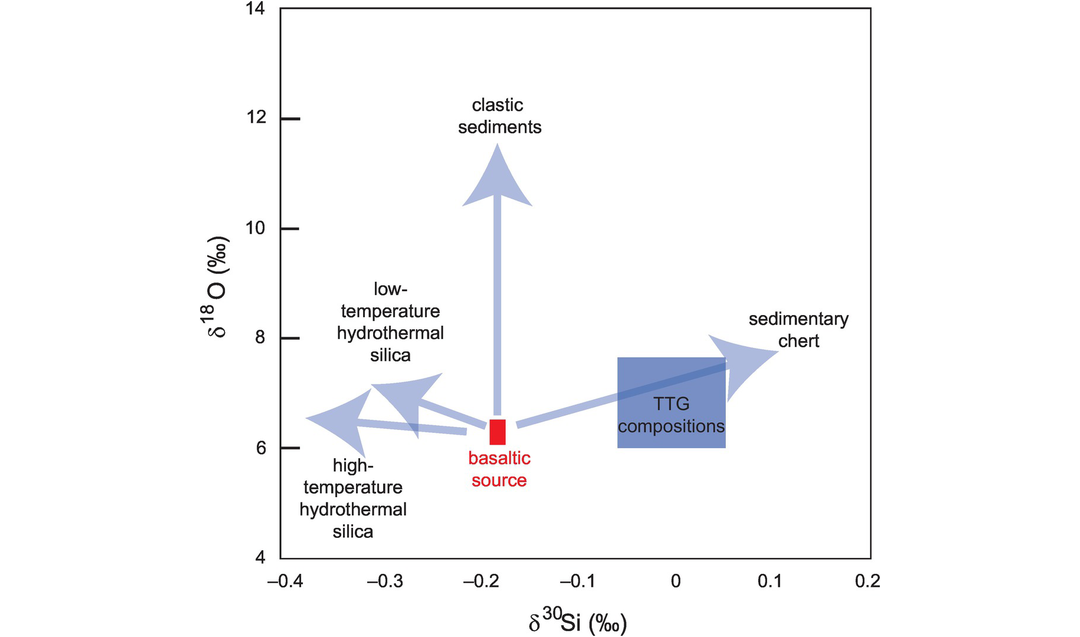
High-resolution silicon versus oxygen isotope diagram showing the likely origin of heavy δ30Si enrichment in Archaean tonalite–trondhemite–granodiorite (TTG) magmas. The diagram shows the influence of different contaminants on the silicon and oxygen isotope composition of a partial melt of a basaltic source (red box) relative to the measured composition of Archaean TTGs.
7.4.4 Chromium Isotopes
Chromium is an important trace element in many igneous rocks. It is most abundant in mafic and ultramafic igneous rocks where it is compatible in ferromagnesian minerals. Cr is also present in the oxide phase chromite (MgFe)Cr2O4, an important accessory phase in mafic and ultramafic rocks and the dominant phase in cumulate chromitite rocks. Chromium is a redox-sensitive element. In most minerals it occurs in the Cr3+ state, although during weathering it may be oxidised to Cr6+. Cr3+ forms oxides or hydroxides which are insoluble; in contrast, Cr6+ is bound with oxygen to form CrO42− chromate, HCrO4− bichromate or Cr2O72− dichromate ions, all of which are water-soluble. Cr6+ is carcinogenic, and because of its soluble nature the anthropogenic Cr contamination of groundwater through industrial activity has led to some serious environmental problems.
There are four stable isotopes of chromium: 50Cr, 52Cr, 53Cr and 54Cr. 53Cr is the daughter product of the now-extinct radionuclide 53Mn. Chromium isotope ratios are measured as 53Cr/52Cr, expressed as δ53Cr‰ (Eq. 7.29) relative to the standard SRM979. In natural systems Cr isotopes have a range of about 7‰ (Figure 7.35); the stable isotope systematics of Cr are summarised in Box 7.12. A recent review of the stable isotope geochemistry of chromium is given by Qin and Wang (2017).
High-precision chromium isotope measurements can be made using thermal ionisation mass spectrometry (TIMS) with a reported precision of up to 0.026‰ and by MC-ICP-MS techniques with a precision of between ±0.26 and 0.011‰. After acid dissolution, samples are purified using ion-exchange techniques. In situ analyses are performed by LA-ICP-MS. A full discussion of analytical approaches is given in Qin and Wang (2017).
Chromium isotopes have been used to study processes in the early solar system, in the redox evolution of the Earth’s early atmosphere and oceans and in environmental geochemistry to investigate contaminated groundwater.
Stable isotopes and abundances
Measured isotope ratios
Standards
SRM979, from the National Institute of Standards and Technology, often denoted as NIST 979; also SRM3112a. Both supplied in Cr3+ form in nitric acid.
NIST610 and NIST612 for LA-ICP-MS (Bai et al., 2019)
Chondritic value
Silicate Earth
Variations in nature
See Figure 7.35.
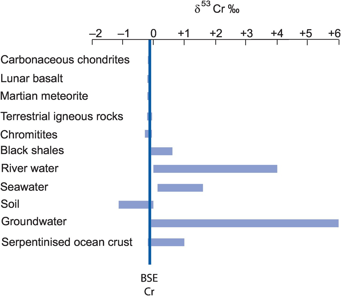
Variation in δ53Cr in extra-terrestrial and terrestrial reservoirs relative to the value of the silicate Earth.
7.4.4.1 The Distribution of Chromium Isotopes in Nature
The average chromium isotope composition of carbonaceous chondrites is δ53Cr = −0.128 ± 0.043‰ and of ordinary chondrites δ53Cr = −0.113 ± 0.044‰. Measurements on two Martian meteorites give values between δ53Cr = −0.218 and −0.142‰ (Schoenberg et al., 2016) and the least differentiated lunar basalt of Bonnand et al. (2016) has a Cr isotopic composition of −0.222 ± 0.025‰.
The chromium isotope composition of mantle-derived rocks is in the range δ53Cr = −0.009 to 0.211‰. For mantle xenoliths δ53Cr values = −0.017 to −0.167‰, for ultramafic rocks and cumulates δ53Cr = −0.009 to −0.211‰ and for oceanic and continental basalts δ53Cr = −0.126 to −0.178‰ (average δ53Cr = −0.151 ± 0.050‰). From these measurements it is possible to estimate an average value for the igneous silicate Earth of δ53Cr = −0.124 ± 0.101‰ (Schoenberg et al., 2008). A single measurement on a USGS granite reference sample gives δ53Cr = −0.177‰, within the range of the mafic igneous rocks measured (Schoenberg et al., 2016), suggesting that an average value for the continental crust is similar to that of the silicate Earth. The similarity between the δ53Cr values for the silicate Earth, Mars and chondritic meteorites suggests that contrary to earlier proposals there was no fractionation of chromium isotopes during core formation in the silicate Earth and Mars.
Farkas et al. (2013) calculated the global average Cr isotope composition for chromites as −0.079 ± 0.169‰. Chromitites in layered intrusions (the Bushveld complex, the Great Dyke, the Stillwater complex) have Cr isotope compositions in the range δ53Cr = −0.23 to −0.026‰ (Schoenberg et al., 2008; Bai et al., 2019). In the Kizildag ophiolite in Turkey, Chen et al. (2019) show that podiform chromitites have slightly heavier δ53Cr values (−0.22 to −0.04‰) than those in ophiolitic stratiform-like chromitites (−0.29 to −0.06‰) indicating that the range of chromium isotope compositions in ophiolitic chromitites is greater than that found in layered intrusions. Currently, all measured chromite Cr isotope compositions lie within the range of values for the silicate Earth.
Marine sediments have δ53Cr values between −0.007 to +0.009 (mean 0.032 ± 0.065). Black shales analysed by Frank et al. (2020) have bulk δ53Cr values of between +0.02 ± 0.15‰ and +0.56 ± 0.10‰ and a chert sample has a bulk δ53Cr value of +0.98 ± 0.13‰.
Chromium in modern river water is predominantly as Cr6+ and is derived from the weathering of the continental crust. River water has chromium isotope compositions ranging from δ53Cr = −0.17 to +1.33‰, although in source regions containing serpentinised ultramafic rocks values may be as high as +4‰ (Farkas et al., 2013). Seawater is not well mixed with respect to Cr isotopes and there is an inverse correlation between the Cr isotope composition and Cr concentrations in seawater (Paulukat et al., 2016). δ53Cr values are between +0.13 and +1.6‰, although in surface waters the range is +0.13 to +1.24‰ (Paulukat et al., 2016; Qin and Wang, 2017).
7.4.4.2 Controls on the Fractionation of Chromium Isotopes
The reduction of Cr6+ to Cr3+ involves the breaking of Cr–O bonds because Cr6+ usually exists as an oxy-anion. The bonds between the light Cr isotopes and oxygen are easier to break than for the heavy isotopes, and so during reducing reactions the Cr3+ product will be enriched in the light Cr isotopes. At low temperatures this kinetic fractionation may take place by both abiotic and biological processes. The abiotic reduction of Cr6+ to Cr3+ in laboratory experiments using a range of mineral substrates results in isotopic fractionations of the order of 2.5–3.5‰. In Fe2+-rich sediments this can lead to an increase in δ53Cr in the overlying water of up to 2.0‰ (Qin and Wang, 2017; Bauer et al., 2018).
Biological Cr6+ reduction by microbial activity is an important process in natural systems, and in the laboratory fractionations from 2.0 to 7.0‰ have been measured. In each case the reduced reaction product is isotopically lighter than the reactant. However, the transfer of three electrons from Cr6+ to Cr3+ is likely to occur in stages and so in natural systems the precise amount of fractionation will depend upon the reduction pathway and may not be as high as that predicted from laboratory experiments. The detail of metabolic pathways in thermophilic bacteria has been documented recently by Chen et al. (2019). In contrast to Cr6+ reduction, the processes whereby Cr3+ is oxidised to Cr6+ are less well understood, but experimental studies indicate Cr isotope fractionations of between −2.5 and +1.0‰ (Qin and Wang, 2017).
The very small (<0.2‰) variations in silicate rocks indicate that Cr isotopes are not extensively fractionated in high-temperature igneous systems. However, Schoenberg et al. (2016) have suggested that within this variability there are some small fractionations which reflect both partial melting and fractional crystallisation processes. This has been confirmed in a recent study by Chen et al. (2019), who demonstrated Cr isotope equilibrium fractionation during partial melting of mantle harzburgite of the Kizildag ophiolite and in the fractional crystallisation of the associated dunites and chromitites. Bai et al. (2019) have shown that during fractional crystallisation, heavy Cr isotopes are preferentially partitioned into chromite and the light isotopes into the residual melt such that equilibrium processes lead to Cr isotopic fractionation between minerals in the order δ53Crspinel > δ53Crorthopyroxene > δ53Crolivine.
In addition to equilibrium fractionation processes, there is also evidence of kinetic fractionation in high-temperature igneous systems. This can be seen in the Stillwater complex in the United States where the Cr isotope composition of olivines shows inter-mineral fractionations which do not follow the sequence identified above, and δ53Cr diffusion profiles in these olivines indicate that kinetic factors play a role in Cr isotope fractionation (Bai et al., 2019).
7.4.4.3 Using Chromium Isotopes as a Tracer in Cosmological and Geological Processes
The isotope 53Cr is produced from the decay of the short-lived isotope 53Mn, which has a half-life of 3.7 Ma. Mass-independent anomalies of 53Cr in meteorites have been used to provide clues about early processes in the solar nebula and the differentiation of early planetesimals. In addition, anomalies of the isotope 54Cr in meteorites can be used to trace the sources and distribution of nucleosynthetic products in the early solar system (see review by Qin and Wang, 2017).
On the Earth the spread of Cr isotope values illustrated in Figure 7.35 shows that the most significant fractionations take place during low-temperature geochemical processes. One such process is the oxidative continental weathering of Cr3+ to Cr6+, although this requires MnO2 as a catalyst and in detail is complex. Where Cr is lost from the system during weathering, the resulting palaeosols show negative δ53Cr values; currently, this weathering process is the only natural mechanism known to produce large negative Cr isotope fractionations (Frei and Polat, 2013). Other soil profiles record Cr enrichment; these have positive δ53Cr values and where the weathering leads to the serpentinization of ultramafic rocks, Cr isotope compositions can be shifted to δ53Cr values as high as 1.2‰ (Farkas et al., 2013).
Cr isotope fractionation in the oceans is driven by two key processes: the reduction of Cr6+ in surface waters and the scavenging of isotopically light Cr3+ to deeper water and sediment. A recent model for the mass balance of Cr isotopes in the modern oceans suggests that the principal Cr input is from rivers with an estimated δ53Cr = +0.3 to +1.0‰. Outputs include relatively minor fluxes of Cr to oxic and anoxic sediments, both with zero δ53Cr fractionation and a major flux to reducing sediments with an estimated δ53Cr fractionation of −0.2. This model is consistent with a Cr isotope composition for the oceans of δ53Cr = +0.44 to +1.53‰ (Qin and Wang, 2017).
In groundwater chromium isotopes can be used to understand the transport of the carcinogenic contaminant Cr6+. In particular, the anaerobic reduction of Cr6+ can immobilise carcinogenic Cr and convert it into insoluble Cr3+. The Cr isotope fractionation associated with this process can lead to elevated δ53Cr values (0.7–5.2‰) and in this way the efficiency of the remediation can be monitored. In detail, the measured Cr isotope values will be very variable for they depend on the initial δ53Cr value of the source and whether it is natural or anthropogenic.
A relatively recent application of Cr isotopes has been to use δ53Cr values in sediments as a palaeo-redox proxy and to determine the onset of oxygenic photosynthesis. This approach has been applied to the study of banded iron formations, organic-rich shales and carbonate rocks. The logic is that in an oxygenated atmosphere Cr can be oxidised to Cr6+, mobilised and isotopically fractionated. In an oxygen-free atmosphere Cr is transported as Cr-bearing minerals or as dissolved Cr3+ but is not fractionated. However, despite this simple theoretical framework, care must be taken to ensure that the sediments analysed faithfully record the ambient δ53Cr for seawater. Consequently, corrections may need to be made for the presence of detrital material in the sediment (Frank et al., 2020) and for any biological Cr isotope fractionations. Further, geochemical controls on the oxidation of Cr require both the presence of Mn oxides, which in itself requires free oxygen, and a surface environment free of Fe2+.
A compilation of δ53Crsediment over geological time for selected samples shows that there is minimal δ53Cr fractionation (−0.5 to +0.5‰) relative to the silicate Earth from the Hadean to the mid-Proterozoic. Only in the Neoproterozoic at ~1.1 Ga is there a record of extensive δ53Cr fractionation (up to +5.0‰ in Fe-rich shales), long after the GOE at 2.34 Ga. This event at 1.1 Ga is thought to record the onset of oxidised surface environments and the deep oxygenation of ocean waters (Qin and Wang, 2017).
7.4.5 Iron Isotopes
The element iron is abundant throughout the Earth. It occurs in three oxidation states – metallic iron (Fe0), ferrous iron (Fe2+) and ferric iron (Fe3+) – and these oxidation states govern its distribution. Metallic iron is the primary constituent of the Earth’s core; ferrous iron is the dominant iron species in the Earth’s mantle and its derivative melts, and ferric iron is common in the oxygenated environments of the Earth’s surface.
There are four stable isotopes of iron: 54Fe, 56Fe, 57Fe and 58Fe. The isotope ratio measured is 56Fe/54Fe, expressed as δ56Fe‰ (Eq. 7.30) relative to a synthetic iron standard. The range of isotopic fractionations in natural samples is about 6.0‰, from ~ −3.5 to +2.7‰. The systematics of iron isotopes are summarised in Box 7.13, and recent reviews of the geochemistry of the stable isotopes of iron are given by Dauphas et al. (2017) and in the text by Johnson et al. (2020). Bulk samples are prepared for analysis using acid digestions followed by element purification using ion-exchange methods. The analytical method of choice is MC-ICP-MS for its precision and speed of analysis, although where high spatial resolution is required, then the in situ methods of SIMS and LA-ICP-MS can be applied. A full discussion of analytical approaches is given in Dauphas et al. (2017) and Johnson et al. (2020).
In igneous rocks only very small shifts in δ56Fe are recorded, but these can be used to interpret melting and crystal fractionation processes. In contrast, in the aqueous environments of the Earth surface, the composition of some sediments and surface waters shows large iron isotope fractionations (Figure 7.36). Iron is also an essential element in living organisms; large isotopic fractionations are recorded in plants, animals and humans; and there are applications of Fe isotope chemistry in biomedical research (Albarede et al., 2017; Dauphas et al., 2017).
Stable isotopes and abundances
Measured isotope ratios
Standards
IRMM-014 (a synthetic metallic iron from the Institute for Reference Materials and Methods)
In practice the standard IRMM-524a is currently used; this has the same Fe isotopic value as IRMM-014
Chondritic value
Bulk silicate Earth value
δ56Fe ~ chondritic (Dauphas et al., 2017)
Variations in nature
See Figure 7.36.
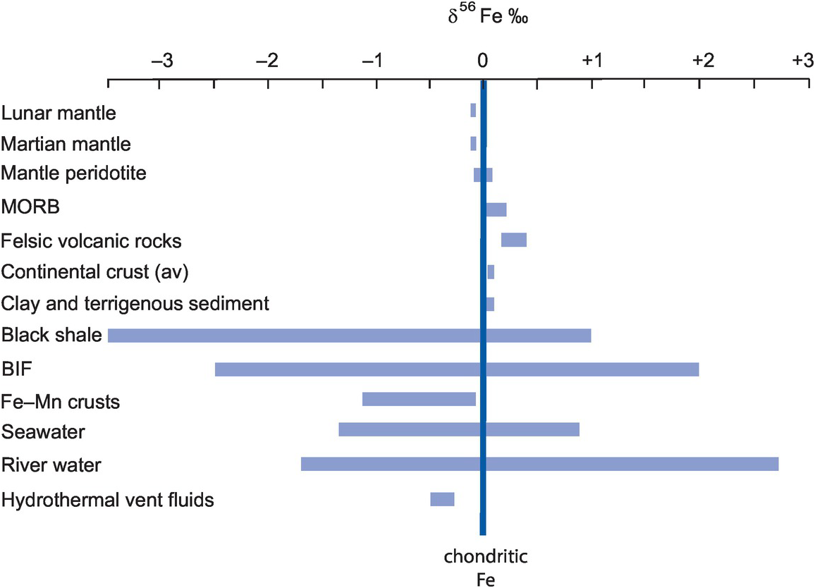
Variation in δ56Fe in extra-terrestrial and terrestrial reservoirs relative to the value in chondritic meteorites, which is identical to the BSE value.
7.4.5.1 The Distribution of Iron Isotopes in Nature
Chondritic meteorites have a mean iron isotope value of δ56Fe = −0.005 ± 0.006‰, a value which is constant throughout all chondrite types, and is coincidentally indistinguishable from that of the iron isotope standard IRMM-014, which is by definition δ56Fe = 0.0. The estimated composition of the Martian mantle is δ57Fe = −0.12 ± 0.04 and the primitive lunar mantle is δ56Fe = −0.10 ± 0.05‰; both are slightly lighter than the chondritic value (Dauphas et al., 2017; Elardo et al., 2019).
Current estimates for the composition of the terrestrial mantle include the average for mantle peridotites of δ56Fe = −0.027 ± 0.026‰ with δ56Fe values ranging from −0.1 to +0.16‰ (Dauphas et al., 2017), and the estimated composition of the Earth’s primitive mantle is δ56Fe = +0.033 ± 0.027‰ (Sossi et al., 2016). Baffin Island picrites are in the range δ56Fe = −0.025 to + 0.125‰, with a parental melt composition of 0.076 ± 0.04‰ (McCoy-West et al., 2018). MORBs have a compositional range of δ56Fe = +0.06 to +0.18‰ with a mean value of +0.105 ± 0.006‰, and a calculated MORB source of +0.025 ± 0.025‰. Estimates of the iron isotope composition of the mantle source for komatiite lavas is between +0.054 to −0.093‰ (summarised in McCoy-West et al., 2018). Arc lavas from the Banda Arc are thought to be derived from a mantle source which has a lower δ56Fe than that of MORB. Taken together, these variations in terrestrial mafic and ultramafic rocks lead to an emerging consensus that the Fe isotope composition of the bulk silicate Earth is chondritic (see review by Dauphas et al., 2017).
δ56Fe values in silicic rocks increase with the increasing silica content of the melt. Below 70 wt.‰ SiO2, δ56Fe values are between +0.08 and +0.14‰, but above 70 wt.‰ SiO2, values increase rapidly to +0.4‰. Poitrasson (2006) computed a mean value for the continental crust of δ56Fe = +0.07 ± 0.03‰ (given as δ57Fe = +0.10 ± 0.03‰).
Values for dissolved δ56Fe in the world’s oceans are variable but show the greatest range in the North Atlantic where they vary between −1.35 ± 0.03‰ and +0.80 ± 0.06‰ (Abadie et al., 2017). The combined dissolved and particulate δ56Fe in river water varies between −1.7 and +2.7‰ (Escoube et al., 2015). High-temperature hydrothermal vent fluids have δ56Fe values in the range −0.3 to −0.5‰, shifted towards lighter values relative to the composition of igneous rocks.
Modern deep-sea clays and terrigenous sediments have δ56Fe values which cluster around the value for average continental crust (δ56Fe = +0.07 ± 0.03‰), indicating that there is only minor iron isotope fractionation during continental weathering and transport. However, sediments formed in organic-rich reducing environments such as black shales show a much wider range with δ56Fe = +1.0 to −3.5‰. Modern marine chemical sediments such as Fe–Mn crusts and nodules are enriched in the light isotopes and have δ56Fe values between −0.05 and −1.13‰ (mean = −0.41 ± 0.49‰). Banded iron formations formed in the Proterozoic and Archaean preserve a wide range of compositions with δ56Fe values between −2.5 and +2.0‰ (Dauphas et al., 2017).
7.4.5.2 Controls on the Fractionation of Iron Isotopes
Evidence for kinetically controlled iron isotope fractionation at high temperatures comes from the study of diffusion in zoned minerals. Teng et al. (2011) measured δ56Fe in a strongly zoned olivine from Kīlauea Iki lava lake and showed that the low-Fe core was isotopically light with δ56Fe ~ −1.0‰, whereas the Fe-enriched rim was isotopically heavier with δ56Fe ~ 0.0‰. Their data suggest that as the melt became more Fe-rich, Fe diffused into the olivine with the light Fe isotopes diffusing into the phenocryst more rapidly than the heavy ones, giving rise to the isotopically light mineral core. At low temperatures, examples of kinetically controlled isotope fractionations have been seen both in experimental studies and in natural systems. Examples include the biological oxidation of Fe, biological and abiotic mineral dissolution, the precipitation of Fe from seawater and the biological uptake of Fe from seawater.
Equilibrium Fe isotope fractionations are quantified using the fractionation factor β, a measure of the fractionation of a given phase relative to monatomic Fe vapour. The use of a reference material in this way allows fractionation factors to be calculated between any two coexisting phases (Dauphas et al., 2017). Experimental studies of Fe isotope fractionation between silicate and metal at high temperatures indicate that the degree of fractionation is very small, confirming the view that the composition of the BSE was little modified during core formation (Elardo et al., 2019). Other high-temperature fractionations include the mineral–melt partitioning (Δ56Fe) between spinel and melt = 0.15–0.22‰ and between olivine and melt = 0.048‰ (McCoy-West et al., 2018). Mineral–mineral fractionation factors for the phases almandine, ilmenite, fayalite, chromite, hercynite and magnetite were determined by Sossi and O’Neill (2017), who showed that both the coordination environment and the oxidation state of the Fe exert important controls on Fe isotope fractionation.
In aqueous solutions the fractionation factor for Fe isotopes between Fe2+ and Fe3+ was determined experimentally by Welch et al. (2003), who showed that the ferrous component is always isotopically light relative to the ferric component. The average measured ΔFe3+–Fe2+ fractionation was +3.57 ± 0.38‰ at 0°C, +3.00 ± 0.23‰ at 22°C and estimated to be +1.5 ± 0.6‰ at 100°C. Measured fractionations between aqueous Fe species and minerals include Fe3+–haematite = −0.1 ± 0.2‰, Fe2+–magnetite = −1.56 ± 0.20‰ at 22oC, Fe2+–siderite = +0.48 ± 0.22‰ at 20°C and Fe2+–mackinawite (FeS) = −0.33 ± 0.12‰ at 25°C (Dauphas et al., 2017, and references therein).
Leaching of Fe from basaltic rocks during hydrothermal alteration results in the release of the lighter isotope such that high-temperature vent fluids are isotopically light and the altered basalt isotopically heavy relative to fresh values by up to 1.3‰. This is due to the formation of isotopically heavy secondary minerals and the precipitation of isotopically heavy pyrite in the basalt. During continental weathering Fe isotope fractionation in soil is small, often less than ~0.5‰, indicating that weathering does not significantly fractionate iron isotopes.
In biogeochemical processes the principal controls on iron isotope fractionation include bacterial dissimilatory iron reduction (DIR) and iron oxidation. During DIR, bacteria use Fe3+ as an electron acceptor in anaerobic respiration – an important process in the formation of sulphide minerals. Experimental studies show that iron isotope fractionation between Fe2+ in solution and a ferric substrate during DIR can lead to δ56Fe values that are up to 2.95‰ lower than that of the substrate, very similar to the values determined by Welch et al. (2003) for the abiotic fractionation of aqueous Fe2+–Fe3+. In contrast, photosynthetic Fe2+-oxidising bacteria, operating under anaerobic conditions and using Fe2+aq as an electron donor, crystallize hydrous ferric oxide enriched in δ56Fe by about 1.5‰. Plants also fractionate iron isotopes relative to soil, with an overall range in fractionation of up to 4.5‰ (see review by Dauphas et al., 2017).
7.4.5.3 Using Iron Isotopes as a Tracer in Geological and Biological Processes
The largest fractionations between the isotopes of iron are to be found in aqueous environments and as a result of biogeochemical processes (Figure 7.36). The balance of iron isotopes in the oceans is controlled by the input of isotopically heavy Fe in aerosol dust and river water, the input of isotopically light hydrothermal vent fluids and pore waters and the biological removal of heavy isotopes (Albarede et al., 2017; Dauphas et al., 2017).
Iron isotopes also serve as a useful proxy for palaeo-redox conditions, for prior to the GOE it is thought that the Earth’s oceans were anoxic and rich in isotopically light δ56Fe. The black shale iron isotope archive shows a wide range of values in samples from the early Proterozoic and the Archaean (δ56Fe = +1.0 to −3.5‰) but a much narrower spread in rocks younger than about 2.3 Ga. This difference is thought to reflect a change in the redox state of the global oceans related to the oxygenation of the Earth’s atmosphere during the GOE at 2.34 Ga. Similarly, there are large iron isotope fractionations in Archaean and Proterozoic banded iron formations (BIF) prior to 1.8 Ga (δ56Fe = −2.5 and +2.0‰), although it is unclear how much of this fractionation is primary and how much is the product of post-depositional processes (Dauphas et al. 2017).
It has been suggested that the extreme iron isotope fractionations in Archaean sediments are, in part, the product of microbial activity, although this is difficult to demonstrate unequivocally since similar fractionations can be produced by abiotic processes. Nevertheless, the recent study by Marin-Carbonne et al. (2020) argues that 3.2 Ga sedimentary pyrites from the Barberton Greenstone Belt in South Africa preserve evidence of microbial activity in the form of dissimilatory iron reduction.
In high-temperature geochemistry the difference between the average iron isotope composition of mantle peridotites (δ56Fe = −0.027 ± 0.026‰) and MORBs (δ56Fe = +0.105 ± 0.006‰) suggests that there is equilibrium iron isotope fractionation during the partial melting of the mantle. This is difficult to quantify, but McCoy-West et al. (2018) propose a δ56Femelt– δ56Fesource value of <0.04‰ for high degrees of mantle melting, although at present not all the relevant mineral–melt fractionation factors are well known (Dauphas et al., 2017). In felsic rocks the steep increase in δ56Fe values with increasing silica content is most likely to be the product of fractional crystallisation, although the initial redox state of the melt and the role of Fe3+ should be also be taken into consideration when evaluating these isotopic fractionations (Teng et al., 2008; Dauphas et al., 2017).